- Research
- Open access
- Published:
Time-order error and scalar variance in a computational model of human timing: simulations and predictions
Computational Cognitive Science volume 1, Article number: 3 (2015)
Abstract
Background
This work introduces a computational model of human temporal discrimination mechanism – the Clock-Counter Timing Network. It is an artificial neural network implementation of a timing mechanism based on the informational architecture of the popular Scalar Timing Model.
Methods
The model has been simulated in a virtual environment enabling computational experiments which imitate a temporal discrimination task – the two-alternative forced choice task. The influence of key parameters of the model (including the internal pacemaker speed and the variability of memory translation) on the network accuracy and the time-order error phenomenon has been evaluated.
Results
The results of simulations reveal how activities of different modules contribute to the overall performance of the model. While the number of significant effects is quite large, the article focuses on the relevant observations concerning the influence of the pacemaker speed and the scalar source of variance on the measured indicators of network performance.
Conclusions
The results of performed experiments demonstrate consequences of the fundamental assumptions of the clock-counter model for the results in a temporal discrimination task. The results can be compared and verified in empirical experiments with human participants, especially when the modes of activity of the internal timing mechanism are changed because of some external conditions, or are impaired due to some kind of a neural degradation process.
Background
Timing is one of the fundamental cognitive abilities among humans and animals. Temporal information is used by living organisms to perform many crucial tasks such as movement, planning and communication. Therefore it is of great importance to gain knowledge on how human timing mechanisms work, what are the biological (and especially neural) bases of these mechanisms, and what are their limitations.
Psychology, psychophysics and neuroscience of human timing have provided many theoretical approaches. One of the prominent approaches are clock-counter models (Eisler 1981; Gibbon 1992; Gibbon et al. 1984; Ulrich et al. 2006; Wearden 1999, 2003; Wearden and Doherty 1995). This class of models revolves around the concept of the internal clock emitting impulses and the counter storing these pulses whenever a stimulus is presented. One of the most popular models of this class is the Scalar Timing Model. Another type of model that has been recently proposed is the state-dependent network model (Buonomano et al. 2009; Karmarkar and Buonomano 2007). This model relies on the idea of a network of simple computational elements, where internal time is encoded as a changing state of neurons during and after exposition of stimuli. Yet another prominent group of models is constituted by psychophysical quantitative models (Church 1999; Getty 1975, 1976; Killeen and Weiss 1987; Rammsayer and Ulrich 2001). These models are usually represented as sets of equations describing dependencies between physical properties of a stimulus and an internal, subjective representation of time. These psychophysical equations are sometimes closely related to the other groups of models, and may be seen as their specification. Apart from these groups of models, there exist more complex interdisciplinary approaches, combining neurological, psychological and computational knowledge (Church 2003; Matell and Meck 2004; Meck 2005). More information on different classes of time perception models is provided in (Buhusi and Meck 2005; Grondin 2001; Ivry and Schlerf 2008; Zakay et al. 1999). Models that are outside of the classification outlined above are described in (Shi et al. 2013; Staddon and Higga 1999; Yamazaki and Tanaka 2005). Overall, these are good theoretical frameworks: they provide explanations to experimental data, some of them are equipped with tools allowing to perform advanced simulations, and some of them integrate knowledge and data from different scientific disciplines. Nevertheless, a unified, commonly accepted theory of human timing is yet to beproposed.
Apart from the development of better and better explanations of human timing processes, much time and resources have also been devoted to explore human (and animal) timing phenomena. There is a great body of research concerning interval timing, ranging from behavioral experiments conducted on animal and human subjects (Gibbon 1977; Grondin 2005; Wearden et al. 2007) to neuroimaging studies and research on patients with mental or neurodegenerative diseases (Grondin 2010; Hairston and Nagarajan 2007; Malapani et al. 1998; Riesen and Schnider 2001; Sévigny et al. 2003; Smith et al. 2007). Among experimental findings, several phenomena have been frequently reported and analyzed. One of them is the scalar property of animal and human timing – a characteristic often perceived as an equivalent of Weber’s law in the domain of timing (Eisler et al. 2008; Wearden and Lejeune 2008; Wearden et al. 1997; Komosinski 2012). Depending on the type of an experiment, the scalar property may denote a constant coefficient of variation of a subject’s timing judgments/measurements when perceiving stimuli of different durations, or a superposition of distributions of estimations of different time intervals, expressed on the same, relative timescale (Church 2002). This property became the core assumption of one of the most popular timing models – the Scalar Timing Model (Gibbon et al. 1984; Wearden 1999, 2003) or STM, which is a part of the Scalar Expectancy Theory – SET. The STM and the SET are popular (Perbal et al. 2005; Wearden et al. 2007) despite the fact that the scalar property is not observed in some experiments (Komosinski 2012; Lewis and Miall 2009; Wearden and Lejeune 2008).
Another frequently reported and robust phenomenon is the time-order error – TOE (Allan 1977; Hairston and Nagarajan 2007; Hellström 1985; Hellström and Rammsayer 2004; Jamieson and Petrusic 1975). The TOE is reported when duration (but also loudness, pitch, weight, etc.) of two successively presented stimuli is compared; this procedure is known as the two-alternative forced choice task (2-AFC). In the domain of human timing it is called the temporal discrimination task.
The TOE is a systematic overestimation (a positive TOE) or underestimation (a negative TOE) of the first stimulus relative to the second one. While the negative TOE is generally more common, many factors influence the magnitude and even the polarity of the TOE. For example, it is often reported that when the intensity of stimuli is low (in a context of timing research they have short durations), the TOE is closer to zero, and it even becomes positive (Allan 1977; Hellström 2003). Another important factor influencing the TOE is an interstimulus interval (ISI); it was reported that longer ISIs cause a decrease of the magnitude of the TOE (Jamieson and Petrusic 1975). Many kinds of explanations have been proposed (Eisler et al. 2008; Hellström 1985), but there is no single explanation that would cover every property of the TOE. What is quite certain is that this is a perception-related phenomenon, not the decision-making one. As much as the TOE is a matter to consider by theoreticians of human timing, it is also a methodological issue. The order of presentation of temporal stimuli may distort the response pattern of participants, increasing or decreasing correct response rate by tens of percent (Jamieson and Petrusic 1975; Schab and Crowder 1988).
Responding to the need for a unified model of human timing, we have implemented an informational architecture of a commonly known clock-counter model, the STM, in a connectionist environment of an artificial neural network (Komosinski and Kups 2009, 2011). We call this implementation the Clock-Counter Timing Network. In order to research the responses of the CCTN we developed a software platform which is able to conduct an artificial behavioral experiment: the temporal discrimination task. The CCTN consists of a number of modules, of which some are adopted directly from the STM. Furthermore, by including a few additional assumptions, the CCTN is able to manifest the TOE. A preliminary computational experiment proved that the CCTN can mimic the behavior of a human (the participant “BJ” from the study of (Allan 1977)). This was possible even though those simulations did not demonstrate the scalar property which, according to various studies, does not always hold; such experiments allowed minimizing the influence of additional sources of variability in the otherwise complex system.
After establishing that the CCTN is able to successfully manifest the TOE, it is natural to ask whether the source of scalar variability in the network affects the TOE and the network’s ability to mimic human behaviors. Answering this question may reveal how the two frequently reported phenomena interact. What is more, including the assumption of the scalar property in the CCTN makes this architecture more similar to the STM, which is the original theoretical foundation of the CCTN.
Results reported in this paper demonstrate that the computational representation of the STM is capable of explaining the robustness of the TOE, and it is also useful in predicting performance in the temporal discrimination task under different modes of activity. These capabilities make the CCTN a valuable contribution in the quest for explaining human timing mechanisms.
The neural model – the clock-counter timing network
To build a neural model of the timing mechanism and to perform the experiments, the Framsticks simulation environment was employed (Hapke and Komosinski 2008; Jelonek and Komosinski 2006; Komosinski and Ulatowski 2009, 2014). Apart from tools designed to build complex neural models, this software is able to efficiently perform simulation and optimization. Since simulation time is measured in simulation steps, it was assumed that one millisecond corresponds to one simulation step.
Neurons
The basic processing units used in the CCTN are depicted in Figure 1. These are artificial neurons processing signal received from inputs and transforming it according to some rule or a simple function:
-
1.
SeeLight – a receptor that outputs a value corresponding to the detected quantity of a stimulus; it can be used as a model of a light, sound, or smell sensor.
-
2.
Pulse – outputs a pulse once in a few simulation steps; the number of steps between pulses is exponentially distributed and the mean can be adjusted.
-
3.
Gate – this neuron has one control input and one or more standard inputs; if a signal flowing through the control input is positive, than the neuron outputs the weighted sum of inputs that have positive weights. When the signal in control input is negative, then the neuron outputs the weighted sum of inputs that have negative weights. For zero control signal the neuron outputs zero.
-
4.
Thr – a threshold neuron with a binary transfer function. The threshold value and both output values can be adjusted.
-
5.
Gauss – outputs a product of the input value and the value drawn from the normal distribution of a given mean and a standard deviation.
-
6.
Sum – accumulates received signals in each step and outputs currently accumulated value,
-
7.
Delay – propagates input to output with an adjustable delay of a number of simulation steps.

Neuron types used in the network shown in Figure 2 . The “Gate” neuron conditionally passes input signal to output, depending on the state of the additional control input. The names of the remaining neurons indicate their function.
Modules in the CCTN
The modules of the CCTN are shown in Figure 2. As described below, these modules belong to two groups: the modules present in the Scalar Timing Model informational architecture and additional modules enabling the CCTN to compare pairs of sequentially presented stimuli.
-
Modules present in the STM:
-
1.
Pacemaker – consists of one Pulse neuron which has no input and emits pulses once in a few steps. The key parameter of this neuron is the mean interpulse interval, further referred to as the Pacemaker Period or the Pacemaker Speed.
-
2.
Switch – consists of one Gate Neuron; lets the signal from the Pacemaker through whenever it receives a positive signal from the Receptor.
-
3.
Accumulator – in the default state it stores the bias signal from the Accumulator Bias Module. When a stimulus is present (the Receptor is excited), the Accumulator stores the pulses from the Pacemaker.
-
4.
Reference Memory – the role of this module is slightly different than in the original STM. The module stores the signal from the Scalar Variance Module after the end of the first stimulus (this information represents the duration of the stimulus). This module is also equipped with the resetting loop which starts to reset the memory after the exposition of the second stimulus. In the original STM, this module integrates lengths of conditional stimuli during the conditional/learning part of the experiment, and during the testing part, a randomly drawn sample of the duration is compared with the information stored in the working memory.
-
5.
Working Memory – stores the signal from the Scalar Variance Module after the end of the second stimulus; it is equipped with a resetting loop which starts to reset it several steps after the signal is stored in memory.
-
6.
Comparator – a few steps after the end of the second stimulus, it compares the values stored in the Reference and Working Memory buffers; if the signal from the Reference Memory has a greater absolute value than the signal from the Working Memory, the Comparator outputs 1.0. In the opposite case, the Comparator outputs −1.0. When the absolute difference between the two signals is lower than 0.1 (which usually happens before the end of a trial, and might happen when the difference between the two signals is really small), the Comparator outputs 0.0.
-
7.
Scalar Variance Module – this module is not an explicit part of the STM, however, the function it serves is one of the ways of producing scalar variance (Komosinski 2012). The module consists of one Gauss neuron which receives signal from the Accumulator, and outputs the product of its input and a random value drawn from the normal distribution with a given mean and a standard deviation. The mean and the standard deviation are further subjected to experimental manipulations, along with other parameters of the CCTN.
-
1.
-
Modules enabling CCTN to compare pairs of stimuli:
-
8.
Stimulus Monitoring Module – consists of one Thr neuron that receives the signal from the Receptor. If the input signal is higher than the arbitrary threshold (currently set to 0.001), the module outputs 1.0, otherwise it outputs 0.0.
-
9.
Accumulator Control Module – it is equipped with its own buffer (a Sum neuron). The module receives signals from the Accumulator Reset Module and the Receptor, and it outputs signals to the Accumulator Reset Module and to the Accumulator Bias Module. The role of the Accumulator Control Module is to recognize when to enable the two modules. The Accumulator Control Module enables the Reset Module after the end of the stimulus, and stops it when the signal in the Accumulator is close to a threshold value (0.1 by default); after that, the Accumulator Control Module enables the Bias Module, which stops on its own when a threshold of the bias value is reached.
-
10.
Accumulator Reset Module – receives signals from the Accumulator Control Module and from the Stimulus Monitoring Module. The main part of this module is a negative feedback loop which starts several steps after the stimulus has ended. The module clears the state of the Accumulator by decreasing the accumulated value so that it may drop even below the bias threshold. The exact moment of stopping the activity of this module is determined by the Accumulator Control Module; the signal value in the Accumulator indicating this moment is called later the Accumulator Reset Lower Bound. The rate at which this module clears the signal in the Accumulator, further referred to as the Accumulator Reset Rate, is equal to the amount of signal that is deducted from the signal stored in the Accumulator.
-
11.
Accumulator Bias Module – receives inputs from the Accumulator Control Module and the Stimulus Monitoring Module. After receiving a proper signal from the Control Module, it outputs a positive value until the signal stored in the Accumulator reaches a certain threshold. The amount of signal added to the signal in the Accumulator is called the Accumulator Bias Recovery Rate. The bias charging threshold is further referred to as Accumulator Bias. The processes of resetting and charging the Accumulator with the bias signal do not overlap.
-
12.
Accumulator-Memory Mediator – receives signals from the Scalar Variance Module, the Reference Memory Module and the End-of-stimulus Module. This module passes the signal to the Reference Memory or to the Working Memory, depending on which stimulus of the pair has been presented.
-
13.
End-of-stimulus Module – receives signals from the SeeLight receptor and the Accumulator Reset Module, and outputs control signals to the Comparator and to the Accumulator-Memory Mediator. Depending on whether the first or the second stimulus ends, this module enables the transfer of the signal from the Accumulator through the Accumulator-Memory Mediator or it enables the comparison process in the Comparator.
-
8.

The CCTN artificial neural network based on the STM architecture; the network compares lengths of two stimuli. Individual modules are described in the text.
An example of the key modules of the CCTN processing signals is shown in Figure 3. The scalar property of timing is provided by the Scalar Variance Module (7). Another way to observe this property would be to use more biologically adequate building elements which may produce the scalar property emergently or to introduce some form of an inherent noise. However, the main goal of this work is to see how scalar property interacts with the TOE phenomenon and not to explain the scalar property itself.

Sample signal waveform in the key modules of the CCTN comparing two pairs of stimuli. Top panel: When the stimuli are presented, the Receptor feeds the 1.0 value to the network. During the presence of the stimulus, the Accumulator collects the signal from the Pacemaker module. After the exposition of each stimulus, the Accumulator Reset Module resets the signal in the Accumulator – the signal in the Accumulator gradually drops. The Scalar Variance Module located between the Accumulator and the memory modules introduces Gaussian noise to the signal sent from the Accumulator. Middle panel: After the exposition of the first/second stimulus of a pair, the Reference/Working Memory stores the signal acquired from the Scalar Variance Module. After the end of a trial, the signal in these memories is reset. Bottom panel: After the end of the second stimulus of a pair, the Comparator compares signals from the Working Memory and the Reference Memory. When the value in the Reference Memory is bigger, the Comparator sends 1.0, otherwise it sends −1.0. Note that in the example shown, the CCTN made an error when comparing the first pair of stimuli: the Comparator sent a positive value while, in fact, the second stimulus lasted longer.
Time-order error in the CCTN
In general, the TOE for two durations can be calculated as the difference between the conditional probability of the correct answer when the first stimulus lasted longer (the “LongShort” case), and the probability of the correct answer when the second stimulus lasted longer (the “ShortLong” case). In the case when the presented stimuli have the same durations, the TOE is calculated as the difference between the frequency of the answer “the first stimulus lasted longer” and 50 percent. To enable proper comparisons of the TOE values in these two different situations, the resulting value in the former case has to be halved (Jamieson and Petrusic 1975). The formulas describing these two measures are:
A negative TOE value means overestimation of the second stimulus relative to the first one, which can be measured as a higher frequency of the correct answer when the second stimulus of a pair lasted longer, than in the case when the stimuli were presented in the reverse order – compare with (1). If the presented stimuli are of the same duration, a negative TOE means that the answer “the second stimulus lasted longer” is more frequent than 50 percent – compare with (2). A positive TOE means that the opposite pattern of responses occurred. As mentioned before, the earlier version of the CCTN that was not equipped with the Scalar Variance Module was capable of manifesting the TOE – at least for the range of stimuli used in the experiment described by Allan (see Section “Data”), and of nearly the same magnitude as the one exhibited by the participant BJ.
A positive TOE occurs mainly due to the activity of the Accumulator Bias Module and the Accumulator Reset Module. If, after the exposition of the first stimulus of a pair, the signal drops below the default level and then the second stimulus appears, the second stimulus has a smaller chance to be reported by the network as being longer than the first one. Increasing length of the interstimulus interval would reduce this effect; this phenomenon is reported in the literature on human timing (Jamieson and Petrusic 1975).
A negative TOE in the CCTN is caused by the work of the Accumulator Reset Module. If, after the exposition of the first stimulus from a pair, there are many pulses accumulated in the Accumulator and the resetting process is slow, then at the time of the arrival of the second stimulus, the Accumulator still contains remnants of the pulses accumulated during the first stimulus. If the remaining value in the Accumulator is higher than the default bias, then there is a greater chance that the second stimulus will be reported as longer. Note that according to the predictions of the CCTN, this effect should be smaller for shorter stimuli and a longer interstimulus interval. Again, these phenomena are reported in the literature on human timing (Jamieson and Petrusic 1975). A sufficiently long interstimulus interval would cause the TOE to be positive, which is a prediction that is yet to be confirmed in a separate empirical experiments.
The basic mechanisms responsible for the TOE that have been proposed in our earlier research remain the same in the present version of the CCTN. The assumptions underlying the manifestation of the TOE have led to the development of the model’s ability to reflect human behaviors in timing tasks. In this work we investigate how including the source of scalar variability influences patterns of neural network responses during temporal discrimination of relatively short stimuli. These stimuli are in the range of tens to less than two hundred milliseconds, although in the experiment concerning variability of temporal representation, longer stimuli were considered as well. The existence of the source of scalar variance is shown to be unable to “swamp” the variance generated by the Poissonian generator when stimuli are really short (Gibbon 1992). This behavior is also supported by empirical data demonstrating that stimuli in the range of milliseconds tend to cause higher coefficients of variation of judgements than longer stimuli, and that the magnitude of this ratio drops fast as the stimuli get longer (Lewis and Miall 2009; Wearden and Lejeune 2008).
Methods
Data
To perform extensive analyses of the CCTN, the idea of an experiment originally performed by Allan (1977) was employed. Allan’s data have been previously used in tasks that model timing mechanisms (Eisler 1981; Hellström 1985). Our experiments imitate the structure of the Experiment II – more specifically, the part where participants compared short stimuli. In this part, subjects were presented with the set of short durations in each trial, and had to decide which of the two visual stimuli lasted longer. The set of stimuli consisted of ten different types of pairs of stimuli ranging from 70 to 160 ms. Apart from adaptation of the experimental procedure, we have also fit the data from simulation experiments to the results of the “BJ” participant. The data were taken from Table two in (Allan 1977) with TOE for unequal stimuli halved to enable direct comparisons with pairs containing equally long stimuli.
Each pair of stimuli was presented to this participant approximately 150 times across 5 sessions of 3 blocks of 100 pairs. Actually, in the case of “BJ”, 1–5 presentations of each pair did not take place or their results were discarded from further analysis (Eisler 1981), but because these numbers were relatively low, this artifact was not reflected in our experiments.
For further analyses, we used the proportions of the responses “first longer” – meaning the the first stimulus of the pair was reported as lasting longer. Such proportions are also provided for each subject and for each stimuli length in the Allan’s study.
Experimental procedures
To investigate the behavior of the CCTN and the interplay between its parameters, two kinds of simulations were performed. The aim of the first one was to study the influence of the Scalar Variance Module on the variability of signals in the Reference Memory and in the Working Memory modules. The second experiment was designed to study the TOE phenomenon and its dependence on parameter values of the network. The crucial part of the second experiment was testing how different parameters of the Scalar Variance Module influence the magnitude of the TOE, the overall accuracy of discrimination of two short stimuli, and the goodness of fit of the network to the human behavior.
The CCTN parameters
In this work, the influence of six important parameters of the CCTN on the actual outcome of the stimuli comparison is studied. These parameters are:
-
Pacemaker Period PP – the mean interval between consecutive pulses in the Pacemaker Module. It is calculated as \(\frac {1}{\lambda }\), where λ is the mean of the Poissonian distribution. The PP parameter is often called the internal clock speed.
-
The mean S V μ and the standard deviation S V σ of the normal distribution used in the Scalar Variance Module. These two parameters are further referred to as the Scalar Variance factor SV, as both values determine the (scalar) variability of stimuli representations in the Working Memory module.
-
The Accumulator Reset Rate ARR – the rate at which the accumulator is cleaned up after exposition of a stimulus. This parameter is highly responsible for the negative TOE, since the remnants of the signal in the Accumulator Module add up to the signal related to the second stimulus and, in consequence, lead to its overestimation. The signal value in the Accumulator module at which the resetting process stops is called the Accumulator Reset Lower Bound, ARLB, and it was constant in our experiments.
-
The Accumulator Bias value AB – the default signal value in the Accumulator when no stimulus is presented. Increasing this value potentially favors positive TOE, as the value may be added to the value which represents the first stimulus in a pair. However, the actual time profile of a trial and the Accumulator Bias Recovery Rate determine whether increased AB would indeed lead to the overestimation of the first stimulus.
-
The Accumulator Bias Recovery Rate ABRR – the rate at which the Accumulator Bias recovers after the exposition of the second stimulus in a pair.
Experiment 1
Ten different CCTN networks were considered; each of them was presented 1000 times with a set of 27 different pairs of identical stimuli. Each network was characterized by one of the five pairs of parameters of the Scalar Variance Module: (S V μ=1.0,S V σ=0.05),(S V μ=1.0,S V σ=0.1),(S V μ=1.0,S V σ=0.2),(S V μ=2.0,S V σ=0.2), and (S V μ=2.0,S V σ=0.4). In each network, the period of the Pacemaker Module was set to either \(\frac {1}{\lambda } = 10\) ss or \(\frac {1}{\lambda } = 20\) ss (ss denotes simulation steps). It was assumed that one ss reflects one millisecond. Other important parameters of the networks were adjusted so that there was no interference in the Accumulator between the signal remaining after the exposition of the first stimulus and the signal related to the second stimulus: the Accumulator Reset Rate A R R=0.005, the Accumulator Reset Lower Bound A R L B=0.1, the Accumulator bias (default signal) A B=0.5, the Accumulator Bias Recovery Rate A B R R=0.001. The stimuli ranged from 10 ss to 10000 ss. Pairs of stimuli were presented in the ascending order of stimulus length. Presentation of each pair was preceded by 2750 ss to charge the Accumulator with the bias signal. The interstimulus interval (ISI) of each pair lasted 10000 ss. Because the main aim of this experiment was to explore the behavior of networks comparing short stimuli, the stimuli in the range 10–280 ss were sampled with the highest resolution (30 ss); stimuli in the range 300–900 ss were sampled every 100 ss, and stimuli in the range 1000–10000 ss were sampled every 1000 ss. During the experiment, the network responded after the exposition of the second stimulus. The absolute difference between the signals from the Reference Memory and the Working Memory had to be higher than 0.01 for the Comparator to send out 1.0 (the first stimulus considered longer), or −1.0 (the second stimulus considered longer); otherwise the Comparator would output 0.0. The time between the end of the second stimulus of a pair and the start of the next trial lasted 3000 ss to let the network return to the initial state.
Experiment 2
270 networks were examined, and each network had a different configuration of six crucial parameters: the period of the Pacemaker Module pulse generation \(\left (\frac {1}{\lambda }\right)\), the mean and the standard deviation of the normal distribution associated with the Scalar Variance Module (S V μ and S V σ), the Accumulator Reset Rate ARR, the Accumulator Bias value AB, and the Accumulator Bias Recovery Rate ABRR. The remaining aspects of network settings were the same as in the Experiment 1. The values of the parameters were as follows: λ∈{1/5,1/10,1/20}, (S V μ,S V σ)∈{(1.0,0.05), (1.0,0.1), (1.0,0.2), (2.0,0.2), (2.0,0.4)}, A R R∈{0.0016, 0.0017, 0.0018, 0.0019, 0.002}, A B∈{0.1,0.6,1.1}, A B R R∈{0.001,0.011}. All the combinations of parameters in these sets yield a total of 216 network configurations. Additionally, networks with no Scalar Variance Module were examined; excluding parameters for scalar variability gives 54 combinations of the remaining parameters, thus 270 networks in total. Each of these networks was tested 32 times.
There were ten different pairs of stimuli lengths given in simulation steps: (70,100), (100,70), (100,130), (130,100), (130,160), (160, 130), (70,70), (100, 100), (130,130), and (160, 160). Each pair was presented to a network 150 times, hence 1500 pairs in total presented to each of the 270 networks. The simulation setup has been arranged to be similar to the experiment conducted by Allan (see Section “Data”) with some obvious differences. Since artificial networks were tested, not humans, the experiment was not divided into blocks and sessions; as the networks were not equipped with sophisticated sensory and decision systems, there were no warning signals at the beginnings of trials, and stimulation concerned a single, simulated receptor.
Data collection and analyses
In the first experiment, values of signals were collected from four key neurons of the network: the Accumulator buffer, the Reference Memory buffer, the Working Memory buffer and the output of the Comparator module. For each network, one thousand values for each type of pair of stimuli were registered for all the modules except the Accumulator, from which we have collected two thousand values related to each of the stimuli. For the first three key neurons the mean value, the standard deviation and the coefficient of variation of the signal were computed. For the Comparator module, the proportion of the “first stimulus longer” signal for each stimuli pair was calculated. Additionally, distributions of the values from the Accumulator, the Reference Memory and the Working Memory were determined for each duration of stimuli. These values were stored during the trials. The values from the Accumulator were collected just after the end of the stimuli, the values from the Reference and the Working Memory buffers were collected several steps after the end of the stimuli, and the output value from the Comparator module was collected after the end of the second stimulus.
In the second experiment, for each network and for each type of stimuli pair, the proportion of the “first stimulus longer” response was calculated from the output of the Comparator. The cases of 0.0 signals (meaning that the difference between signals from the Reference Memory and the Working Memory was too small) were randomly assigned to one of the two categories. Having these proportions, the ratios of the correct answers for each stimuli pair and the TOE values were determined. For each pair of stimuli, we have also calculated the mean squared error (MSE) between response rates of the network and the participant BJ (see Section “Data”). Statistical analyses were performed using the IBM SPSS Statistics package, version 21.0.0.1.
Results
Experiment 1
Figure 4 demonstrates that for each set of parameters of the Scalar Variance Module and the Pacemaker Module, the coefficient of variation of signal values in each memory buffer increased when registered stimuli were shorter than 2000 ss (the results were almost identical for the Working Memory and the Reference Memory buffers, so charts are presented only for the former buffer).

Coefficient of variation (vertical axis) of the signal related to the representation of stimuli duration in the Experiment 1. Left panel: the Accumulator buffer. Right panel: the Working Memory buffer. Gray lines illustrate experiments with Pacemaker speed P P=10, and black lines correspond to P P=20. Three kinds of markers (dot, cross, circle) are used for different S V σ/S V μ ratios. The key is the same for both plots.
Contrary to the Accumulator, in the memory buffers the coefficient of variation stabilized when the duration of stimuli exceeded 2000–4000 ss. In the Accumulator, the coefficient of variation seemed to continuously drop, though the magnitude of the decrease tended to get lower when longer stimuli were presented. A detailed theoretical analysis of this relationship including asymptotic behavior can be found in (Komosinski 2012). Altogether, the coefficient of variation in the Accumulator was higher when the Pacemaker speed was lower (recall that there were only two Pacemaker speeds tested). Although the coefficient of variation in memory buffers was highly influenced by the activity of the Scalar Variance Module, the dependence of the coefficient of variation on the Pacemaker speed was especially visible when the presented stimuli lasted shortly. To see this dependence, compare changes of the coefficient of variation in networks characterized by P P=10, S V σ=0.1, S V μ=1.0 or P P=10, S V σ=0.2, S V μ=2.0 and the network with P P=20, S V σ=0.05, S V μ=1.0. Not surprisingly, the coefficient of variation grew together with the S V σ/S V μ ratio in the Scalar Variance Module, which is especially visible for longer stimuli. A high relative variability added by the Scalar Variance Module accompanied by the increased Pacemaker speed led to a faster stabilization of the coefficient of variation (cf. discussion on Weber’s law in (Komosinski, 2012)).
Apart from signals in the Accumulator and in the memory buffers, we also examined patterns of answers of the networks. For longer stimuli, for each network, two responses favoring one of the stimuli were equally probable. For pairs of the shortest stimuli, however, the answer “do not know” (the Comparator output was 0.0) appeared more often: the absolute difference between the stimuli was below the threshold. The probability of such situations increased with a decreasing speed of the Pacemaker and with the decrease of the relative variability in the Scalar Variance Module.
Experiment 2
Accuracy
The first indicator of timing performance that was measured was the overall accuracy (OA) – the mean percentage of the correct answers for all trials, including differing stimuli.
The outcome of the Kolmogorov-Smirnov test for normality (D=0.007,p=.200) as well as the visual inspection of the Q-Q plot and the histogram showed that the residuals of the dependent variable were consistent with a normal distribution; the outcome of Levene’s test indicated (F=1.361,p<.001) that variances in groups are not homogeneous – which should deem parametric analyses of the dependent variable unusable until the scale is transformed. However, after the arcsin transformation (which caused the results of Levene’s test to be non-significant: F=1.115, p=.099), the output from the 5-way General Linear Model for the transformed data was very similar to the output from non-transformed data: the set of significant effects did not change. The magnitude of the effects on the transformed scale expressed as partial eta squared – \(\mathrm {{\eta _{p}^{2}}}\) was usually slightly higher, but the order of magnitude of the effects was preserved. Because of this behavior and to avoid unnecessary transformations, the results of analyses will be presented for non-transformed data. All post hoc analyses were performed using the Bonferroni testa. The results of the analyses are presented in Table 1.
The main effects of the Scalar Variance factor (S V,\(F(4,8370)=3566, p<.001, \mathrm {{\eta _{p}^{2}}}=.630\)), Pacemaker period factor (\(PP, F(2,8370)=38548, p<.001, \mathrm {{\eta _{p}^{2}}}=.902\)), Accumulator reset rate (\(ARR, F(2,8370)=947, p<.001, \mathrm {{\eta _{p}^{2}}}=.185\)) and Accumulator bias (\(AB, F(2,8370)=233, p<.001, \mathrm {{\eta _{p}^{2}}}=.053\)) were significant. The main effect of the Accumulator bias recovery rate factor was not significant (\(ABRR, F(1,8370)=0.037, p=.847, \mathrm {{\eta _{p}^{2}}}<.001\)).
Post-hoc analyses revealed that for each main effect excluding the SV factor, each pair of levels differed significantly (all p<.001). As for the main effect of SV, all pairs but one (1,0.1-2,0.2: p=.812) differed significantly (p<.001). The details (see also Figure 5) are presented below:
-
PP: the lower was the PP value, the higher was the accuracy.
Figure 5 
Significant main effects on total accuracy of unequal pairs comparison in Experiment 2. Error bars indicate 95% confidence intervals.
-
SV: the highest accuracy was observed for the networks which did not have the scalar source of variability; then the accuracy dropped with the increase of the relative variability produced by the SV module (the networks with the same SV-related variability did not differ significantly).
-
ARR: the increase of the ARR parameter value entailed growth of the OA.
-
AB: a similar trend was observed as in the previous case, however, the growth of the accuracy was less pronounced.

Additionally, there were significant interactions: P P×S V (F(8,8370)=337, p<.001, \(\mathrm {{\eta _{p}^{2}}}=.244\)), P P×A R R (F(4,8370)=206, p<.001, \(\mathrm {{\eta _{p}^{2}}}=.090\)), P P×A B (F(4,8370)=41.9, p<.001, \(\mathrm {{\eta _{p}^{2}}}=.020\)), S V×A R R (F(8,8370)=4.17, p<.001, \(\mathrm {{\eta _{p}^{2}}}=.004\)), S V×A B (F(8,8370)=7.36, p<.001, \(\mathrm {{\eta _{p}^{2}}}=.007\)), A R R×A B (F(4,8370)=10.6, p<.001, \(\mathrm {{\eta _{p}^{2}}}=.005\)), A B×A B R R (F(2,8370)=3.03, p=.049, \(\mathrm {{\eta _{p}^{2}}}=.001\)), S V×P P×A R R (F(16,8370)=4.18, p<.001, \(\mathrm {{\eta _{p}^{2}}}=.008\)), S V×P P×A B (F(16,8370)=1.69, p=.041, \(\mathrm {{\eta _{p}^{2}}}=.003\)). All the other interactions were not significant (all p≥.109). Most of the interactions were ordinal.
More detailed analyses of interaction effects revealed that (see Figures 6 and 7):
-
P P×S V: networks with lower scalar variability, including the networks without scalar variance source, demonstrated higher accuracy than those with a higher variability. Almost all differences between networks with different SV parameter values were significant across all levels of the PP factor, except for the (1.0,0.5 – non-scalar) pair, P P=20, where p=.027, all other p<.001. The only non-significant difference across all levels of PP was for the (1.0,0.1 – 2.0,0.2) pair: p≥.990. In general, the SV effect was more pronounced when the Pacemaker was faster; the least sensitive to the increase in the Pacemaker speed were the networks with the highest ratio of the S V σ/S V μ in the Scalar Variance Module: the higher the pacemaker speed, the lower the increase of accuracy in these networks.
Figure 6 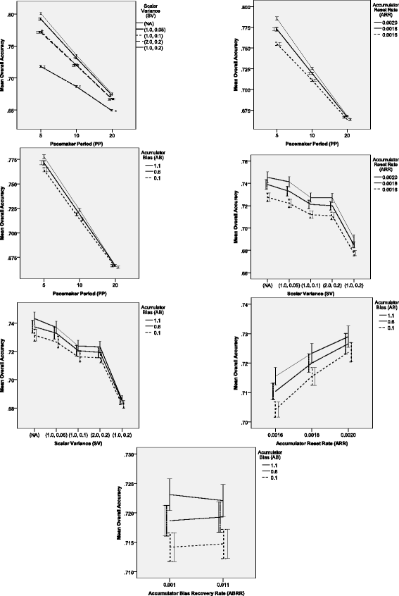
Significant two-way interaction effects on total accuracy of unequal pairs comparison in Experiment 2. Error bars indicate 95% confidence intervals.
Figure 7 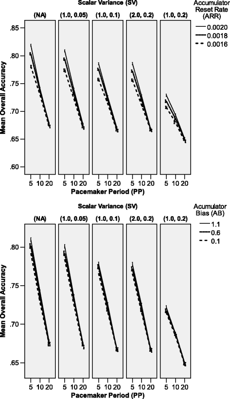
Significant three-way interaction effects on total accuracy of unequal pairs comparison in Experiment 2. Error bars indicate 95% confidence intervals.
-
P P×A R R: except for the lowest speed of the Pacemaker module, pairwise comparisons revealed significant differences (p<.001) between all groups of networks across different Accumulator reset rates. For the lowest values of the PP factor, the only non-significant difference was between networks with the highest and the medium reset rate (p=.063). Other than that, all pairwise differences were significant (p<.001). The OA increased together with the ARR factor values across different levels of the PP factor. The magnitude of the difference changed across different levels of the period factor showing that the difference was higher when the Pacemaker was faster.
-
P P×A B: here the pattern was similar to the previous interaction, except that for the lowest Pacemaker speed, the only significant difference was between two peripheral values of the bias parameter (p=.046). Other differences at this level of the PP factor were not significant (p≥.113).
-
S V×A R R: all differences between values of the ARR across all levels of the SV factor were significant (p<.001) demonstrating that networks with a higher Accumulator reset rate were more accurate than those with lower ARR values. The interaction seemed to be carried out by slight changes in the magnitude of differences between networks with different ARR levels across lower levels of the SV (including the lack of the scalar variance source) and networks with higher levels of the SV.
-
S V×A B: this interaction seemed to be caused by a decreasing discrepancy in accuracy between networks with different Accumulator bias levels (a higher bias level increased accuracy) for growing scalar variability levels (starting from the lack of scalar variability source). Moreover, for the group with the highest relative variability caused by the SV module, the difference between 0.6 and 1.1 levels of the AB factor was non-significant (p=.794).
-
A R R×A B: pairwise comparisons revealed that across all levels of the ARR factor, each pair of groups with different values of the AB parameter differed significantly (p<.001). However, these differences tended to be a bit smaller among the groups with higher values of the ARR parameter. Nevertheless, when the value of the ARR parameter was fixed, then accuracy increased as the value of the AB parameter increased.
-
A B×A B R R: this interaction barely crossed the threshold of statistical significance both before and after the arcsin transformation of the data (p=.049 in both cases), so these results should be treated with caution. The pairwise comparisons revealed (all p<.001) that the discrepancy in accuracy between A B=0.1 and A B=1.1, and between A B=0.6 and A B=1.1 increased slightly when the value of the ABRR factor decreased.
-
S V×P P×A R R: the P P×A R R interaction was modulated by the SV factor – i.e., the difference between networks with a different value of the ARR parameter within the group of the fastest networks was higher when the relative variability was lower (despite the fact that in these cases all p<.001). Across all levels of the SV factor, when the PP was higher than 20, the networks with a higher Accumulator reset rate were more accurate than those with a lower reset rate. Interestingly, as revealed by the F-tests, the effect of the ARR factor was not significant when S V=(2.0,0.2) and P P=20 (p=.375), contrary to all other cases, where p≤.003. There was also a minor non-linearity in the ARR effect size in the medium pacemaker speed groups across levels of the SV factor; overall, the performance dropped as the scalar variability increased.
-
S V×P P×A B: particularly within the group of networks with a lower scalar variability produced by the SV module (or lack thereof), it was observed that the higher the Pacemaker rate, the higher the differences between networks with distinct values of the AB parameter. As revealed by the F-tests, the effect of the AB factor among the networks with the slowest Pacemaker was not significant (p≥.076) across almost all levels of the SV factor; only the networks with the lowest scalar variability (1.0,0.5) differed significantly in this group (p=.016). Apart from that, across all levels of the SV factor, when the PP level was fixed, networks with a higher Accumulator bias were more accurate – however, the overall performance decreased as the scalar variability increased.


TOE
To aggregate results concerning the TOE for different classes of pairs of stimuli, the arithmetic mean of TOE values was calculated across all types of pairs (both with unequal and equal stimuli within a pair). Obviously, this aggregating measure is insufficient to reveal the exact patterns of changes of the TOE across different pairs of stimuli, which are interesting and complex by themselves. However, since all pairwise correlations between the TOE related to different types of pairs were significant, positive and relatively high (all p<.001 and Pearson’s r(8640)≥.717), employing such a measure was justified. To additionally ensure that the mean reflects values of its arguments, only those effects were interpreted that are significant for the majority of TOEs related to individual types of pairs. This time both assumptions of normality of residuals (Kolmogorov-Smirnov test: D=0.007,p=.200) and homogeneity of variances (Levene’s test: F=1.070,p=.208) were met, so all analyses were straightforwardly performed using the GLM and post hoc analyses (the Bonferroni test) on the mean TOE (denoted as mT below). The results of these analyses are presented in Table 2.
All the main effects were significant (\(PP: F(2,8370)=61228, p<.001, \mathrm {{\eta _{p}^{2}}}=.936\); \(SV: F(4,8370)=1216, p<.001, \mathrm {{\eta _{p}^{2}}}=.368; ARR: F(2,8370)=17763\), p<.001, \(\mathrm {{\eta _{p}^{2}}}=.809; AB: F(2,8370)=22313\), p<.001, \(\mathrm {{\eta _{p}^{2}}}=.842\); ABRR: F(1,8370)=37.1, p<.001, \(\mathrm {{\eta _{p}^{2}}}=.004\)). All of these effects were significant for the majority of pair-specific TOEs.
Post-hoc analyses revealed that for each main effect excluding the SV factor, each pair of levels differed significantly (all p<.001). As for the main effect of the SV factor, all pairs but one (1,0.1-2,0.2: p=1.0) differed significantly (p<.001). The mTs averaged for each group of networks were below zero. Details (see Figure 8) are presented below:
-
PP: the higher was the PP value, the lower was the mT (recall that “lower” means more distant from 0.0 and closer to −0.5 – the maximal negative TOE).
Figure 8 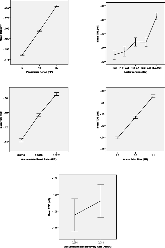
Significant main effects on the mean TOE for all types of comparisons of pairs in Experiment 2. Error bars indicate 95% confidence intervals.
-
SV: the lowest mT was observed for networks which did not have the scalar source of variability; then the mT increased with the growth of the relative scalar variability in the SV module. Networks with the same relative variability of the SV did not differ significantly in the mT.
-
ARR: the increase of the ARR value entailed growth of the mT.
-
AB: the growth of the AB parameter yielded increase of the mT.
-
ABRR: the higher value of the ABRR entailed only slightly a higher mT than the lower value of the ABRR.

The significant interactions were: P P×S V (F(8,8370)=339, p<.001, \(\mathrm {{\eta _{p}^{2}}}=.245\)), P P×A R R (F(4,8370)=291, p<.001, \(\mathrm {{\eta _{p}^{2}}}=.122\)), P P×A B (F(4,8370)=1490, p<.001, \(\mathrm {{\eta _{p}^{2}}}=.416\)), S V×A R R (F(8,8370)=40.4, p<.001, \(\mathrm {{\eta _{p}^{2}}}=.037\)), S V×A B (F(8,8370)=13.6, p<.001, \(\mathrm {{\eta _{p}^{2}}}=.013\)), A R R×A B (F(4,8370)=15.5, p<.001, \(\mathrm {{\eta _{p}^{2}}}=.007\)), P P×S V×A R R (F(16,8370)=3.03, p<.001, \(\mathrm {{\eta _{p}^{2}}}=.006\)), P P×S V×A B (F(16,8370)=2.66, p<.001, \(\mathrm {{\eta _{p}^{2}}}=.005\)), S V×A R R×A B (F(16,8370)=4.42, p<.001, \(\mathrm {{\eta _{p}^{2}}}=.008\)), and P P×S V×A B×A B R R (F(16,8370)=1.77, p=.029, \(\mathrm {{\eta _{p}^{2}}}=.003\)). All the other interactions were not significant (all p≥.063). Not all of these interactions were confirmed by the pair-specific TOE analyses (see below). Most interactions were ordinal.
More detailed analyses of interaction effects revealed that (see Figures 9 and 10):
-
P P×S V: most of the time, when the PP level was fixed, the mT increased with the scalar variability level (starting from the situation when there was no SV module at all). For P P=5 and P P=10, the only non-significant difference was between networks with the same relative variability produced by the SV module (all p=1.0 in these cases; in all other cases, p≤.017). The discrepancy between the mT values within a group of networks with a different relative variability got higher as the Pacemaker speed increased, which was inter alia caused by a drastic slowdown of the mT decreasing rate for the networks with the highest scalar variability. Consistently with this trend, within the networks with P P=20, the only significant differences were between networks with the highest relative variability and with the the remaining levels of SV (all p≤.002; in other cases all p≥.055).
Figure 9 
Significant two-way interaction effects on the mean TOE for all types of comparisons of pairs in Experiment 2. Error bars indicate 95% confidence intervals.
Figure 10 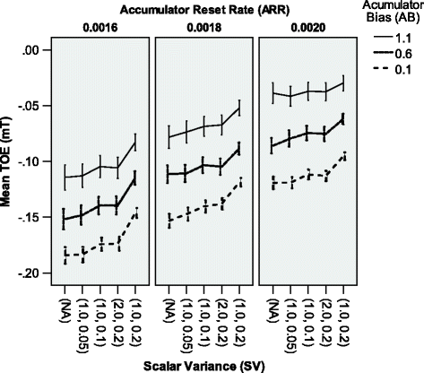
Significant three-way interaction effect on the mean TOE for all types of comparisons of pairs in Experiment 2. Error bars indicate 95% confidence intervals.
-
P P×A R R: all pairwise comparisons within the ARR factor across all levels of the PP factor yielded significant differences (all p<.001), where mT increased with the Accumulator reset rate. The magnitude of the differences between the ARR levels increased with the growing speed of the Pacemaker.
-
P P×A B: all pairwise comparisons within the AB factor across all levels of the PP factor yielded significant differences (all p<.001), where mT increased with the growing value of the Accumulator bias parameter. The magnitude of the differences between the ARR levels decreased with the growing speed of the Pacemaker.
-
S V×A R R: all pairwise comparisons within the ARR factor across all levels of the SV factor yielded significant differences (all p<.001), where mT increased together with the growth of the ARR parameter value. This interaction seemed to be carried out mainly by the visible decrease of the ARR effect when the scalar variance was thehighest.
-
S V×A B: here the pattern was similar to the previous case, however the strength of the effect was slightly lower.
-
A R R×A B: all pairwise comparisons within the AB factor across all levels of the ARR factor yielded significant differences (all p<.001) – the mT decreased as the value of the AB parameter decreased. The differences of mT between different values of the AB parameter seem similar, yet a slight drop of the mT is visible for decreasing ARR for the extreme values of the AB.
-
S V×P P×A R R: this interaction was not significant for TOEs observed for most pairs of stimuli.
-
P P×S V×A B: this interaction was not significant for TOEs observed for most pairs of stimuli.
-
A R R×S V×A B: the interaction between these three factors is easier to interpret when considering ARR as the main modulating factor. As revealed by the F-test, the effect of the AB factor was significant across all levels of the SV factor across all levels of the ARR factor (all p<.001). The increasing Accumulator reset rate seemed to strengthen the S V×A B interaction. When the Accumulator reset rate was low, changes of the mT across the SV levels were quite similar in different levels of the AB factor (though similarly as for other levels of the ARR, the mT was negative all the time and increased with an increase in the bias value). When the Accumulator reset rate was high, the increase of accuracy related to the growth of the relative variability caused by the Scalar Variance module tended to get noticeably smaller as the Accumulator bias value increased.
-
S V×P P×A B×A B R R: this interaction was not significant for TOEs observed for all pairs of stimuli.


Discussion
As the number of significant effects is quite large, the following discussion focuses on the relevant observations concerning the influence of the pacemaker speed and the scalar source of variance on the measured indicators of network performance. These parameters are of the highest importance because the internal clock speed and the memory transfer process are of particular interest in research on human timing. They are also highly influential on the response pattern in the presented version of the 2-AFC task. Other factors are more difficult to be directly operationalized in empirical experiments with human participants without additional low-level empirical research. Nevertheless, complex interactions between the two main factors and the rest of the parameters provide predictions concerning accuracy of the answers of networks and concerning the TOE in the temporal discrimination task. The results obtained from the simulations show the relationship between the human timing mechanism and the exact response patterns in a specific experimental situation. The easiest way to verify predictions of the CCTN without resorting to neuropharmacological manipulations or neuroimaging techniques would be to perform exhaustive timing experiments using a rich set of stimuli and ISIs, and to observe patterns of changes in performance across different types of trials. Such experiments are the next step of our investigation.
Accuracy
The fundamental indicator of performance of networks is the mean proportion of correct answers (OA) across 6 types of trials concerning differing stimuli.
Pacemaker speed
The OA increased with the decreasing pulse generation period of the Pacemaker. The influence of this parameter was modulated by the Accumulator Reset Rate – as the reset rate increased, so did both the value of the OA and the increase of the OA caused by the decreasing PP. Similarly, the growth of the Accumulator Bias strengthened the influence of the PP on the OA. The effect of the PP was not modulated by the Accumulator Bias Recovery Rate. The influence of the PP was also modulated by the value of the Scalar Variance Module parameters – starting from the condition when there was no such module, the higher the relative variability produced by the Scalar Variance Module, the slower the growth of the OA with the decreasing PP. The same S V σ/S V μ ratio of the Scalar Variance Module yielded similar results.
Scalar variance module
Most of the interactions including the SV factor revealed the same pattern: increasing variability related to the Scalar Variance Module diminished the positive influence of the other factors on accuracy. The levels of the factors that increased accuracy more than others (e.g., the levels of PP and AB) often suffered greater loss of the OA. For most of the time, values of the SV parameters yielding the same S V σ/S V μ ratio influenced accuracy in the same way.
As the interaction S V×P P×A R R was significant, the P P×A R R interaction strength (recall that this interaction means that the joint growth of the generator period and the Accumulator reset rate resulted in the greatest increase of accuracy) was diminished by the increase of the relative variability caused by the Scalar Variance Module. The other significant three-way interaction (which is on the verge of significance), S V×P P×A B, was due to a weakening difference in the increase of accuracy between networks differing in Accumulator biases, with a growing PP and with an increasing relative variability of the Scalar Variance Module. This means that the interaction between the PP and the AB parameters is, again, reduced by the growth of the relative variability in the scalar module.
One conclusion from these analyses is that the overall accuracy depends strongly on the pacemaker speed. Although the influence of this parameter was modulated by other parameters, the direction was always the same. This result is important – it means that the increase in the Pacemaker speed yielded the overall increase in accuracy. This is despite the fact that the growing Pacemaker speed should have generally favored the correct answers in the ShortLong order of presentation, and should have lead to decrease of accuracy when the stimuli were presented in the LongShort order. A closer look at the accuracy in the LongShort and the ShortLong orders of presentation revealed that the ShortLong accuracy was higher than the LongShort accuracy, and that the discrepancy between them increased as the Pacemaker speed increased (Figure 11). The LongShort accuracy increased slightly when the Pacemaker was the fastest – this is probably a stimuli-range dependent effect. Additionally, changes of accuracy for the LongShort order were modulated by the Accumulator reset rate and by the ABRR and AB factors. Thus in the investigated range of stimuli, an increase in the Pacemaker speed yielded an interesting effect of an increase of the overall accuracy with the simultaneous increase of the negative TOE.

Mean accuracy presented separately for Short-Long and Long-Short pairs across all levels of the PP factor. Error bars indicate 95% confidence intervals.
The high variability introduced by the Scalar Variance Module was able to dominate the activity of other modules. This, in turn, resulted in the decrease of the overall accuracy in the considered range of stimuli.
TOE
Pacemaker speed
The mean TOE decreased with the growth of the Pacemaker speed. This pattern of changes was modulated by all other factors except for the Accumulator Bias Recovery Rate, ABRR. Two mechanisms of which one is closely related to the positive TOE (the AB factor) and the other is more associated with the establishment of the negative TOE (the ARR factor) yielded the inverse pattern of interactions with the PP: the effect of the AB factor was more pronounced when the Pacemaker speed was lower relatively to the other Pacemaker speed levels – the effect of the ARR factor was stronger when the pacemaker speed was higher. This is consistent with our predictions of the CCTN behavior: when the pacemaker speed is high, a higher signal value should be accumulated in the Accumulator buffer, which means that the proportional contribution of the Accumulator bias drops. At the same time, the rate of the resetting mechanism plays an important role as there is always the same, limited time (ISI) to clean the Accumulator. When the Pacemaker speed is low, the situation is reversed. The influence of the PP on the mT was also modulated by the SV factor as in the case of accuracy: the greater was the scalar variance, the less steep was the growth of the negative mT with the increasing pacemaker speed. Groups of networks with the same S V σ/S V μ ratio yielded almost identical patterns.
Scalar variance
Increasing scalar variance (starting from networks not equipped with the SV module) tended to diminish the effects of other factors decreasing the mT. The two groups of networks equipped with the Scalar Variance modules with the same S V σ/S V μ ratio usually yielded similar results. The interaction effects show that networks which made the lowest mT were most sensitive to the changes in scalar variability produced by the SV module (mT usually increased in these cases).
The only complex interaction that was significant for the majority of the pair-specific TOEs, A R R×S V×A B, reveals that increasing the Accumulator reset rate leads to the growth of the S V×A B strength. At the highest Accumulator reset rate, networks with the highest Accumulator bias value tended to differ less across different levels of the scalar variance. This is probably because when both responses occur equally frequently, increasing variance does not change much. Conversely, when one type of response is prevalent, increasing scalar variability equalizes the proportion of both types of responses. This explains why this interaction may be present when the stimuli are of equal duration in trials. Regarding processing of differing stimuli pairs, as it was shown for accuracy (see Section “Scalar variance module”), usually the correct response rate was higher in the ShortLong than in the LongShort order of presentation. This is not surprising given that the negative mean TOE was prevalent in the results. What is more, on average, the correct response rate for the LongShort order was higher than 50% (M=62.7%, S D=5.1%). This means that increasing the Accumulator reset rate and increasing the Accumulator bias value should have boosted accuracy for the LongShort order above 50%, at the same time decreasing the ShortLong accuracy. Therefore, increasing the Accumulator Bias AB was not only responsible for the increase of the mean TOE. Within the group of networks with the highest Accumulator Reset Rate, it also increased similarity between the two orders of presentation of stimuli in the way accuracy changes for increasing scalarvariability.
Summarizing these remarks, the CCTN model produced results consistent with predictions regarding the examined stimuli range. Increasing the Pacemaker speed acted in favor of producing the negative TOE, and two out of the remaining three TOE generating parameters – ARR and AB – influenced the TOE inversely. The weak influence of the ABRR parameter may mean that the Accumulator bias recovery process rarely occurred. This is in agreement with the observation that a negative mT was prevalent in the collected data. However, as the main effect of the ABRR factor was significant, the predictions concerning the ABRR were confirmed: a higher Accumulator bias charging rate resulted in a slightly increased mT. As for the SV parameter, similarly as in the case of the measured accuracy, an increase in scalar variance resulted in a decrease of other effects. This is caused by the fact that a high scalar variance fosters similarity of memory representations of the first and the second stimulus. The three-way interaction revealed that the increasing contribution of the SV module is not simply additive with effects of other mechanisms. This contribution enables convergence of the accuracy of answers to 50% in both orders of presentation.
Accuracy vs. TOE
The presented results suggest that there is an interesting relation between the TOE and the total accuracy established by the CCTN. The results of the analyses revealed that increasing the pacemaker speed resulted in a lower TOE and in a higher accuracy. On the other hand, increasing the scalar variability caused a decrease in accuracy and in the TOE. To investigate the nature of the relation between the TOE and the OA, additional correlation analysis was performed. This time, the mean TOE for trials consisting of unequal stimuli (mTu) was calculated. The results of this analysis confirmed that there is a negative correlation between the mTu and the OA (p<.001 and Pearson’s r(8640)=−.513). The reason for this may be a higher influence of the relation between mTu and OA for the ShortLong pairs th an for the LongShort pairs. Further analyses revealed that although correlations between the mTu and the OA were opposite, in the ShortLong group the correlation was stronger (p<.001 and Pearson’s r(8640)=−.881) than in the LongShort group (p<.001 and Pearson’s r (8640)=.556). This once again shows that modifying parameters of the timing mechanism does not influence processing of temporal stimuli symmetrically in these two orders of presentation. More importantly, the consequence of this asymmetry is a beneficial impact of the mechanisms responsible for the TOE on the overall quality of temporaljudgements.
Conclusions
The results of performed experiments demonstrate consequences of the fundamental assumptions of the clock–counter model for the results in a temporal discrimination task. We showed that the CCTN is able to model internal timing processes including the scalar variance property. We examined the behavior of a number of neural networks during the temporal discrimination task. The outcome of this study is a set of predictions which can be verified straightforwardly in empirical research. The timing literature proves that a lot of effort is devoted to test how changes in modes of activity of the timing mechanism can change behaviors of humans in the timing task (Meck 2005; Meck and Benson 2002; Wieneret al. 2010). This influence is inter alia tested in experiments that concern Parkinson’s Disease (Artieda et al. 1992; Hellström et al. 1997; Koch et al. 2008; Merchant et al. 2008; Malapani et al. 1998; Malapani et al. 2002; Rammsayer and Classen 1997; Smith et al. 2007), mental disorders (Penney et al. 2005; Sévigny et al. 2003), the influence of drug application (Lustig and Meck 2005; Meck 1983; 1996; Rammsayer 1999), and presentation of stimuli in different modalities (Melgire et al. 2005; Penney et al. 2000; Ulrich et al. 2006). Some of the these works suggest that anatomical correlates of the internal clock are present in basal ganglia and other brain structures connected to this important part of the dopaminergic system (Coull et al. 2008; Coull et al. 2010; Macar et al. 1999; Meck 2006; Perbal et al. 2005).
Such research emphasizes the need for a model which is able to integrate experimental data, to explain obtained results, and finally, to predict patterns of responses in situations that have not been tested empirically. The CCTN model and the simulation results presented in this work demonstrate how the clock speed and other timing mechanism manipulation may influence accuracy and time-order error in the temporal discrimination task. Since it is possible to manipulate the Pacemaker speed (and it is also possible to find patients with impaired Pacemaker speed), the predictions of our model concerning this property of the timing mechanism can be fully verified in empirical experiments. What is more, we investigated a range of parameters of one of the possible sources of the scalar variance proposed in (Gibbon et al. 1984) – the source that is responsible for the memory transfer from the Accumulator module. There is evidence suggesting that memory storage may be unsettled in people with Parkinson’s Disease (Malapani et al. 1998; Malapani et al. 2002). One of the several interesting predictions stemming from our research is that the slowdown of the memory transfer, when it is accompanied by the increase in the relative variability, may reduce the overall accuracy and the magnitude of the time-order error in the temporal discrimination task; this can be verified in PD patients.
Apart from quantitative and qualitative analyses of changes of performance indicators, data fitting analyses have been performed. We are well aware that the proposed model has many free parameters, however it was still important to verify whether it had the potential to reproduce human behavior. The results of the BJ participant (Allan 1977) were used as an example of human characteristics. As the CCTN demonstrated a similar pattern and for some parameters closely resembled experimental data (Figure 12), this is an indication that the model has the potential to be a good explanatory platform for human timing mechanisms. Interestingly, specific analyses revealed that the mean MSE dropped with the increase of the relative scalar variance produced by the SV module (though the differences in MSE were small, see Figure 13), which further emphasizes the importance of the scalar property in timing.

TOE values provided by the CCTN neural networks (270 gray lines, each line is averaged from 32 simulations of a network with a single set of parameters) and provided by a single experiment with a human subject, BJ. The dashed line illustrates a hypothetical situation of zero TOE.

The main effect of the scalar variability factor on the mean squared error (MSE) in Experiment 2. Error bars indicate 95% confidence intervals.
Each of the 270 gray lines shown in Figure 12 shows an average across 32 runs with the same set of parameter values. Since the BJ participant took the experiment only once, a direct comparison between human and simulation data is limited. It is still worth noting that the trend of changes in TOE is consistent for all averaged runs, thus the model can and does simulate empirical reality.
While the CCTN is able to explain more effects than just the influence of stimuli duration on the TOE, our experiments were designed to avoid effects other than those related to stimuli duration. Modeling across-trials effects could be achieved easily, but it would complicate the behavior of the model, while the goal of this work was to isolate and study stimuli duration effects exclusively.
Developing a complete model of human timing is a difficult task; this work demonstrated how to represent a clock-counter timing model in a connectionist architecture. Simulation results prove that the model is a suitable tool to analyze the influence of the scalar sources of variability on temporal judgements, which makes it a descendant of the Scalar Timing Model. Simulations concerning the time-order error phenomenon demonstrated that our model is not only able to manifest it, but also that the manifestation of the TOE may resemble the behavior of a human. This justified investigating interactions between the scalar variance and the TOE – the two hardwired properties of human timing.
There are some analogies between the CCTN and the Sensation Weighting Model (Hellström 2003): in both models, the magnitude of the first or the second stimulus is “strengthened” depending on the context. Our further work will concern the analysis of the recently discovered Type B TOE phenomenon (Dyjas and Ulrich 2014; Ulrich and Vorberg 2009), the exploration of the ISI effect, and the presentation of the results in terms of Just Noticeable Differences instead of raw frequencies of answers. Another issue is the employment of more sophisticated methods of analysis of temporal behaviors, such as adaptive psychophysical procedures – i.e., one of the versions of the up-down procedure (Kaernbach 1991; Leek 2001). To gain more specific knowledge about the stimuli comparison process, simulations will be performed in order to establish determinants of discrimination thresholds or psychometric functions (Wichmann and Hill 2001) related to perception of durations.
Since there are many free parameters in the CCTN, we are going to perform extensive fitting of the proposed model to human data. We would also like to transform the model into the representation consisting only of the integrate-and-fire neurons. Such a representation may cause some of the inherent properties of timing to emerge spontaneously (Buhusi and Oprisan 2013), and it would be a good compromise between the classical clock-counter models and the neural models that have been gaining more and more attention recently. This would meet the need for a connectionist model of timing, fitted to both behavioral and neurobiological data, but still allowing one to comprehend the activity of the network – thus preserving the explanatory power of classical models of timing and at the same time maintaining biological adequacy. This will open a path for further exploration of the patterns of temporal judgements in a wide range of experimental situations.
Endnote
aAs this work concerns simulations with many free parameters and the number of their values is arbitrary, we use a conservative post hoc test to show that the significance of observed effects is not incidental.
References
Allan, LG (1977). The time-order error in judgments of duration. Canadian Journal of Psychology, 31(1), 24–31.
Artieda, J, Pastor, MA, Lacruz, F, Obeso, JA (1992). Temporal discrimination is abnormal in Parkinson’s disease. Brain, 115(1), 199–210.
Buhusi, CV, & Oprisan, SA (2013). Time-scale invariance as an emergent property in a perceptron with realistic, noisy neurons. Behavioural Processes, 95, 60–70. doi:10.1016/j.beproc.2013.02.015.
Buhusi, CV, & Meck, WH (2005). What makes us tick? Functional and neural mechanisms of interval timing. Nature Reviews Neuroscience, 6(10), 755–765.
Buonomano, DV, Bramen, J, Khodadadifar, M (2009). Influence of the interstimulus interval on temporal processing and learning: testing the state-dependent network model. Philosophical Transactions of the Royal Society B, 364, 1865–1873.
Church, RM (1999). Evaluation of quantitative theories of timing. Journal of the Experimental Analysis of Behavior, 71(2), 253–256.
Church, RM (2002). A tribute to John Gibbon. Behavioural Processes, 57, 261–274.
Church, RM (2003). A concise introduction to scalar timing theory. In: Meck, WH (Ed.) In Functional and Neural Mechanisms of Interval Timing. CRC Press, Boca Raton, Florida, (pp. 3–22).
Coull, JT, Nazarian, B, Vidal, F (2008). Timing, storage, and comparison of stimulus duration engage discrete anatomical components of a perceptual timing network. Journal of Cognitive Neuroscience, 20(12), 2185–2197.
Coull, JT, Cheng, R-K, Meck, WH (2010). Neuroanatomical and neurochemical substrates of timing. Neuropsychopharmacology, 36(1), 3–25.
Dyjas, O, & Ulrich, R (2014). Effects of stimulus order on discrimination processes in comparative and equality judgements: Data and models. The Quarterly Journal of Experimental Psychology, 67(6), 1121–1150.
Eisler, H (1981). Applicability of the parallel-clock model to duration discrimination. Attention, Perception, & Psychophysics, 29(3), 225–233.
Eisler, H, Eisler, AD, Hellström, Å (2008). Psychophysical issues in the study of time perception. In: Grondin, S (Ed.) In Psychology of Time. Emerald Group Publishing Ltd, (pp. 75–110).
Getty, DJ (1975). Discrimination of short temporal intervals: A comparison of two models. Perception & Psychophysics, 18(1), 1–8.
Getty, DJ (1976). Counting processes in human timing. Attention, Perception, & Psychophysics, 20, 191–197. ISSN 1943-3921. http://dx.doi.org/10.3758/BF03198600.
Gibbon, J (1977). Scalar expectancy theory and Weber’s law in animal timing. Psychological Review, 84(3), 279–325.
Gibbon, J (1992). Ubiquity of scalar timing with Poisson clock. Journal of Mathematical Psychology, 35, 283–293.
Gibbon, J, Church, RM, Meck, WH (1984). Scalar Timing in Memory. Annals of the New York Academy of Sciences, 423(1), 52–77.
Grondin, S (2001). From physical time to the first and second moments of psychological time. Psychological Bulletin, 127(1), 22–44.
Grondin, S (2005). Overloading temporal memory. Journal of Experimental Psychology: Human Perception and Performance, 31(5), 869–879.
Grondin, S (2010). Timing and time perception: A review of recent behavioral and neuroscience findings and theoretical directions. Attention, Perception, & Psychophysics, 72(3), 561–582.
Hairston, IS, & Nagarajan, SS (2007). Neural mechanisms of the time-order error: An MEG study. Journal of Cognitive Neuroscience, 19(7), 1163–1174.
Hapke, M, & Komosinski, M (2008). Evolutionary Design of Interpretable Fuzzy Controllers. Foundations of Computing and Decision Sciences, 33(4), 351–367. http://www.framsticks.com/files/common/Komosinski_EvolveInterpretableFuzzy.pdf.
Hellström, Å, Lang, H, Portin, R, Rinne, J (1997). Tone duration discrimination in Parkinson’s disease. Neuropsychologia, 35(5), 737–740.
Hellström, Å (1985). The time-order error and its relatives: Mirrors of cognitive processes in comparing. Psychological Bulletin, 97(1), 35–61.
Hellström, Å (2003). Comparison is not just subtraction: Effects of time- and space-order on subjective stimulus difference. Perception & Psychophysics, 65(7), 1161–1177.
Hellström, Å, & Rammsayer, TH (2004). Effects of time-order, interstimulus interval, and feedback in duration discrimination of noise bursts in the 50- and 1000-ms ranges. Acta Psychologica, 116, 1–20.
Ivry, RB, & Schlerf, JE (2008). Dedicated and intrinsic models of time perception. Trends in Cognitive Sciences, 12(7), 273–280.
Jamieson, DG, & Petrusic, WM (1975). The dependence of time-order error direction on stimulus range. Canadian Journal of Psychology, 29(3), 175–182.
Jelonek, J, & Komosinski, M (2006). Biologically-inspired Visual-motor Coordination Model in a Navigation Problem. In: Bogdan, G, Robert, H, Lakhmi, J (Eds.) In Knowledge-Based Intelligent Information and Engineering Systems, volume 4253 of Lecture Notes in Computer Science. http://www.framsticks.com/files/common/BiologicallyInspiredVisualMotorCoordinationModel.pdf. Springer, Berlin/Heidelberg, (pp. 341–348).
Kaernbach, C (1991). Simple adaptive testing with the weighted up-down method. Perception & Psychophysics, 49, 227–229.
Karmarkar, UR, & Buonomano, DV (2007). Telling time in the absence of clocks. Neuron, 53(3), 427.
Killeen, PR, & Weiss, NA (1987). Optimal timing and the Weber function. Psychological Review, 94(4), 455–468.
Koch, G, Costa, A, Brusa, L, Peppe, A, Gatto, I, Torriero, S, Gerfo, EL, Salerno, S, Oliveri, M, Carlesimo, GA (2008). Impaired reproduction of second but not millisecond time intervals in Parkinson’s disease. Neuropsychologia, 46(5), 1305–1313.
Komosinski, M (2012). Measuring quantities using oscillators and pulse generators. Theory in Biosciences, 131(2), 103–116. http://dx.doi.org/10.1007/s12064-012-0153-4.
Komosinski, M, & Kups, A (2009). Models and implementations of timing processes using Artificial Life techniques. Technical Report RA-05/09, Poznan University of Technology, Institute of Computing Science.
Komosinski, M, & Kups, A (2011). Implementation and Simulation of the Scalar Timing Model. Bio-Algorithms and Med-Systems, 7(4), 41–52.
Komosinski, M, & Ulatowski, S (2009). Framsticks: Creating and Understanding Complexity of Life. In: Komosinski, M, & Adamatzky, A (Eds.) In Artificial Life Models in Software, chapter 5, second edition. Springer, London, (pp. 107–148).
Komosinski, M, & Ulatowski, S (2014). Framsticks Web Site. http://www.framsticks.com.
Leek, MR (2001). Adaptive procedures in psychophysical research. Perception & Psychophysics, 63(8), 1279–1292.
Lewis, PA, & Miall, RC (2009). The precision of temporal judgement: milliseconds, many minutes and beyond. Philosophical Transactions of the Royal Society B, 364(2), 1897–1905.
Lustig, C, & Meck, WH (2005). Chronic treatment with haloperidol induces deficits in working memory and feedback effects of interval timing. Brain and Cognition, 58(1), 9–16.
Macar, F, Vidal, F, Casini, L (1999). The supplementary motor area in motor and sensory timing: evidence from slow brain potential changes. Experimental Brain Research, 125(3), 271–280.
Malapani, C, Rakitin, B, Levy, R, Meck, WH, Deweer, B, Dubois, B, Gibbon, J (1998). Coupled temporal memories in Parkinson’s disease: a dopamine-related dysfunction. Journal of Cognitive Neuroscience, 10(3), 316–331.
Malapani, C, Deweer, B, Gibbon, J (2002). Separating storage from retrieval dysfunction of temporal memory in Parkinson’s disease. Journal of Cognitive Neuroscience, 14(2), 311–322.
Matell, MS, & Meck, WH (2004). Cortico-striatal circuits and interval timing: coincidence detection of oscillatory processes. Cognitive Brain Research, 21, 139–170.
Meck, WH (1983). Selective adjustment of the speed of internal clock and memory processes. Journal of experimental psychology. Animal Behavior Processes, 9(2), 171–201.
Meck, WH (1996). Neuropharmacology of timing and time perception. Cognitive Brain Research, 3(3), 227–242.
Meck, WH (2005). Neuropsychology of timing and time perception. Brain and Cognition, 58(1), 1–8.
Meck, WH (2006). Frontal cortex lesions eliminate the clock speed effect of dopaminergic drugs on interval timing. Brain research, 1108(1), 157–167.
Meck, WH, & Benson, AM (2002). Dissecting the brain’s internal clock: how frontal–striatal circuitry keeps time and shifts attention. Brain and Cognition, 48(1), 195–211.
Melgire, M, Ragot, R, Samson, S, Penney, TB, Meck, WH, Pouthas, V (2005). Auditory/visual duration bisection in patients with left or right medial-temporal lobe resection. Brain and Cognition, 58(1), 119–124.
Merchant, H, Luciana, M, Hooper, C, Majestic, S, Tuite, P (2008). Interval timing and Parkinson’s disease: heterogeneity in temporal performance. Experimental Brain Research, 184(2), 233–248.
Penney, TB, Gibbon, J, Meck, WH (2000). Differential effects of auditory and visual signals on clock speed and temporal memory. Journal of Experimental Psychology: Human Perception and Performance, 26(6), 1770–1787.
Penney, TB, Meck, WH, Roberts, SA, Gibbon, J, Erlenmeyer-Kimling, L (2005). Interval-timing deficits in individuals at high risk for schizophrenia. Brain and Cognition, 58(1), 109–118.
Perbal, S, Deweer, B, Pillon, B, Vidailhet, M, Dubois, B, Pouthas, V (2005). Effects of internal clock and memory disorders on duration reproductions and duration productions in patients with Parkinson’s disease. Brain and Cognition, 58(1), 35–48.
Rammsayer, T, & Classen, W (1997). Impaired temporal discrimination in Parkinson’s disease: temporal processing of brief durations as an indicator of degeneration of dopaminergic neurons in the basal ganglia. International Journal of Neuroscience, 91(1-2), 45–55.
Rammsayer, T, & Ulrich, R (2001). Counting models of temporal discrimination. Psychonomic Bulletin & Review, 8(2), 270–277.
Rammsayer, TH (1999). Neuropharmacological evidence for different timing mechanisms in humans. The Quarterly Journal of Experimental Psychology: Section B, 52(3), 273–286.
Riesen, JM, & Schnider, A (2001). Time estimation in Parkinson’s disease: normal long duration estimation despite impaired short duration discrimination. Journal of neurology, 248(1), 27–35.
Schab, FR, & Crowder, RG (1988). The role of succession in temporal cognition: Is the time-order error a recency effect of memory?. Perception & Psychophysics, 44(3), 233–242.
Sévigny, M-C, Everett, J, Grondin, S (2003). Depression, attention, and time estimation. Brain and Cognition, 52(2), 351–353.
Shi, Z, Church, RM, Meck, WH (2013). Bayesian optimization of time perception. Trends in Cognitive Sciences, 17(11), 556–564. doi:10.1016/j.tics.2013.09.009.
Smith, JG, Harper, DN, Gittings, D, Abernethy, D (2007). The effect of Parkinson’s disease on time estimation as a function of stimulus duration range and modality. Brain and Cognition, 64(2), 130–143.
Staddon, JER, & Higga, JJ (1999). Time and memory: Towards a pacemaker-free theory of interval timing. Journal of Experimental Psychology: Animal Behavior Processes, 71(2), 215–251.
Ulrich, R, Nitschke, J, Rammsayer, T (2006). Crossmodal temporal discrimination: Assessing the predictions of a general pacemaker-counter model. Perception & Psychophysics, 68(7), 1140–1152.
Ulrich, R, & Vorberg, D (2009). Estimating the difference limen in 2AFC tasks: Pitfalls and improved estimators. Attention, Perception, & Psychophysics, 71(6), 1219–1227.
Wearden, JH, & Lejeune, H (2008). Scalar properties in human timing: Conformity and violations. The Quarterly Journal of Experimental Psychology, 61(4), 569–587.
Wearden, JH, Denoyan, L, Fakhri, M, Haworth, R (1997). Scalar timing in temporal generalization in humans with longer stimulus durations. Journal of Experimental Psychology: Animal Behavior Processes, 23(4), 502–511.
Wearden, JH (1999). Beyond the fields we know...: exploring and developing scalar timing theory. Behavioural Processes, 45, 3–21.
Wearden, JH (2003). Applying the scalar timing model to human time psychology: Progress and challenges. In: Helfrich, H (Ed.) In Time and mind II: Information processing perspectives. Hogrefe & Huber Publishers, Cambridge, Massachusetts, (pp. 21–39).
Wearden, JH, & Doherty, MF (1995). Exploring and developing a connectionist model of animal timing: Peak procedure and fixed-interval simulations. Journal of Experimental Psychology: Animal Behavior Processes, 21(2), 99–115.
Wearden, JH, Norton, R, Martin, S, Montford-Bebb, O (2007). Internal clock processes and the filled-duration illusion. Journal of Experimental Psychology: Human Perception and Performance, 33(3), 716–729.
Wichmann, FA, & Hill, NJ (2001). The psychometric function: I. Fitting, sampling, and goodness of fit. Perception & psychophysics, 63(8), 1293–1313.
Wiener, M, Hamilton, R, Turkeltaub, P, Matell, MS, Coslett, HB (2010). Fast forward: supramarginal gyrus stimulation alters time measurement. Journal of Cognitive Neuroscience, 22(1), 23–31.
Yamazaki, T, & Tanaka, S (2005). Neural modeling of an internal clock. Neural computation, 17(5), 1032–1058.
Zakay, D, Block, RA, Tsal, Y (1999). Prospective duration estimation and performance. In: Gopher, D, & Koriat, A (Eds.) In Attention and Performance XVII. MIT Press, Cambridge, Massachusetts, (pp. 557–580).
Acknowledgments
This work has been supported by the Polish National Science Centre, grant no. N N519 441939. Computations were performed on the equipment funded by the Polish Ministry of Science and Higher Education, grant no. 6168/IA/128/2012.
Author information
Authors and Affiliations
Corresponding author
Additional information
Competing interests
The authors declare that they have no competing interests.
Authors’ contributions
MK developed the simulation environment and neural simulation scripts. He provided ideas on modeling and simulation of the time-order error, performed theoretical analyses, and guided the development and simulation of the artificial neural network model. AK was responsible for the design of the research; he carried out the simulation studies, data acquisition, statistical analyses and interpretation of the results. Apart from that he drafted the manuscript. Both authors read and approved the final manuscript.
Rights and permissions
Open Access This article is distributed under the terms of the Creative Commons Attribution 4.0 International License (https://creativecommons.org/licenses/by/4.0), which permits use, duplication, adaptation, distribution, and reproduction in any medium or format, as long as you give appropriate credit to the original author(s) and the source, provide a link to the Creative Commons license, and indicate if changes were made.
About this article

Cite this article
Komosinski, M., Kups, A. Time-order error and scalar variance in a computational model of human timing: simulations and predictions. Comput Cogn Sci 1, 3 (2015). https://doi.org/10.1186/s40469-015-0002-0
Received:
Accepted:
Published:
DOI: https://doi.org/10.1186/s40469-015-0002-0