Computation in networks

Abstract

We present an introduction to the modeling of networks of nodes which parse the information presented to them into an output. One example is the nodes are excitable neurons which are collected into a nervous system for an animal whether invertebrate or vertebrate. We will focus on the development of the ideas and tools that might help us understand how to build a model of such a system being careful to explain the many approximations or model errors we make along the way. We start with a discussion of low level biophysical concepts such as the cable equation and the Hodgkin - Huxley model and end with graph based models of computation. We also include motivational arguments that show hardware and software issues in neural models are interwined.

Review

In this article, we will discuss some of the principles behind models of biological information processing. As usual, we therefore use tools at the interface between science, mathematics and computer science. We want to find the right abstraction of the wealth of biological detail that is available; the right design to guide us in the development of our modeling environment. The details of how proteins interact, how genes interact and how neural modules interact to generate the high level outputs we find both interesting and useful are known to some degree but it is quite difficult to use this detailed information to build models of high level function. In all models of this type, we are asking high level questions and wondering how we might create a model that gives us some insight. All such models have built in assumptions and we must train ourselves to think abut these carefully. We must question the abstractions of the messiness of reality that led to the model and be prepared to adjust the modeling process if the world as experienced is different from what the model leads them to expect. There are three primary sources of error when we build models. First, there is the error we make when we abstract from reality; we make choices about which things we are measuring are important. We make further choices about how these things relate to one another. Perhaps we model this with mathematics, diagrams, words etc; whatever we choose to do, there is error we make. This is called Model error. Then, we make error when we use computational tools to solve our abstract models which is called Truncation error. Finally, since we can not store numbers exactly in any computer system, there is always a loss of accuracy because of this. This is called Round Off error. All three of these errors are always present and so the question is how do we know the solutions our models suggest relate to the real world? We must take the modeling results and go back to original data to make sure the model has relevance.

With all this said, let’s start looking at the fundamental building blocks of information transmission in a living neural system. The neurotransmitters and other signaling molecules to accomplish coordination of effort between individual cells were laid down probably in Cambrian times, so these pathways are very old. However, control of a multi-cellular organism such as ourselves does not necessarily require a neural architecture like ours. Recent work in the Ctenophore genome has shown us a new neural architecture for control (see (Moroz et al. 2014), (Callaway 2014), (Staff 2013) and (Ryan et al. 2013)). Also, single cells can be controlled in what appears to be the same way a multi-cellular organism can be as is seen in the video (Nautilus 2014). This implies our framework for understanding how to build useful neural architectures for our goals (understanding cognition, drug treatment, autonomous movement and so forth) does not have to be tied to the architectures we see in invertebrate and vertebrate animals. This implies we are not limited to ideas from invertebrate and vertebrate physiology to solve problems in computational cognition modeling.

The physical laws of ion movement

We start with a simple cell and ion movement in and out of the cell ((Johnson and Wu 1995), (Weiss 1996a) and (Weiss 1996b)). These references provide even more detail and you should feel free to look at these books. However, the amount of detail in them can be overwhelming, so we offer a short version with just enough detail for our mathematical/ biological engineer and computer scientist audience.

An ion c can move across a membrane due to several forces. First, let’s talk about what concentration of a molecule means. For any molecule b, the concentration of the ion is denoted by the symbol [b] and is measured in $\frac {molecules}{liter}$. Now, we hardly ever measure concentration in molecules per unit volume; instead we use the fact that there are N _A =6.02 × 10²³ molecules in a Mole and usually measure concentration in the units $\frac {Moles}{cm^{3}} \: = M$ where for simplicity, the symbol M denotes the concentration in Moles per c m ³. The special number N _A is called Avogadro’s Number. The force that arises from the rate of change of the concentration of molecule b acts on the molecules in the membrane to help move them across. The amount of molecules that move across per unit area due to this force is labeled the diffusion flux as flux is defined to a rate of transfer $\left (\frac {something}{second}\right)$ per unit area.

There are several basic laws to consider. Ficke’s Law of Diffusion is an empirical law which says the rate of change of the concentration of molecule b is proportional to the diffusion flux and is written in mathematical form as $J_{\textit {diff}} = - D \: \frac {\partial \: [b]}{\partial x}$ where J _diff is diffusion flux which has units of $\frac {molecules}{cm^{2}-second}$, D is the diffusion coefficient which has units of $\frac {cm^{2}}{second}$ and [b] is the concentration of molecule b which has units of $\frac {molecules}{cm^{3}}$. The minus sign implies that flow is from high to low concentration; hence diffusion takes place down the concentration gradient. Note that D is the proportionality constant in this law.

Ohm’s Law of Drift relates the electrical field due to an charged molecule, i.e. an ion, c, across a membrane to the drift of the ion across the membrane where drift is the amount of ions that moves across the membrane per unit area. In mathematical form J _drift =− ∂ _el E where it is important to define our variables and units very carefully. We have J _drift is the drift of the ion which has units of $\frac {molecules}{cm^{2}-second}$ and ∂ _el is electrical conductivity which has units of $\frac {molecules}{volt-cm-second}$. Now the valence of ion c is the charge on the ion as an integer; i.e. the valence of C l ⁻ is −1 and the valence of C a ⁺² is +2. We let the valence of the ion c be denoted by z. It is possible to derive the following relation between concentration [c] and the electrical conductivity ∂ _el :∂ _el =μ z [c] where dimensional analysis shows us that the proportionality constant μ, called the mobility of ion c, has units $\frac {cm^{2}}{volt-second}$. Hence, we can rewrite Ohm’s Law of Drift as $J_{\textit {drift}} = - \mu z [c] \: \frac {\partial V}{\partial x}$. We see that the drift of charged particles goes against the electrical gradient.

There is also a relation between the diffusion coefficient D and the mobility μ of an ion which is called Einstein’s Relation. It says $D = \frac {\kappa T}{q} \: \mu$ where κ is Boltzmann’s constant which is $1.38 \: 10^{-23} \frac {joule}{\circ K}$, T is the temperature in degrees Kelvin and q is the charge of the ion c which has units of coulombs. We note electrical work has units of coulombs - volts. Hence, we see $\frac {\kappa T}{q} \: \mu$ has units $\frac {volt-coulomb}{\circ K} \: \frac {\circ K}{coulombs} \: \frac {cm^{2}}{volt-second} \: = \: \frac {cm^{2}}{sec}$ which reduces to the units of D. Further, we see that Einstein’s Law says that diffusion and drift processes are additive because Ohm’s Law of Drift says J _drift is proportional to μ which by Einstein’s Law is proportional to D and hence J _diff .

The membrane capacitance of a typical cell is one micro fahrad per unit area. Typically, we use F to denote the unit fahrads and the unit of area is c m ². Since the inside and outside of the cell are separated by a biological membrane of the type, we can ask what if one side of the cell had more or less ions than the other? These uncompensated ions would produce a voltage difference across the membrane because charge is capacitance times voltage (q = c V). Hence, if we wanted to produce a 100 mV potential difference across the membrane, we can compute how many uncompensated ions, δ[c] would be needed: $\delta [c] = \frac {10^{-6}F}{cm^{2}} \: \times \:.1 V = \: 10^{-7} \: \frac {coulombs}{cm^{2}}$. This is a typical voltage difference across a biological membrane in an excitable nerve cell. For a typical cell the total number of ions inside the cell for a.5M solution is ≈10¹⁶ ions. We can show the number of uncompensated ions per cell to get this voltage difference is 4.95 × 10⁷ ions which is only ≈ 10⁻⁷ % of the total. Hence, the voltage differences relevant to excitable nerve cell are achieved by moving a tiny fraction of the ions available across the membrane.

The Nernst - Planck equation

Under physiological conditions, ion movement across the membrane is influenced by both electric fields and concentration gradients. Let J denote the total flux, then we will assume that we can add linearly the diffusion due to the molecule c and the drift due to the ion c giving J=J _drift + J _diff Thus, applying Ohm’s Law of Drift and Ficke’s Law, we have $J = -\mu \: z \: [\!c] \: \frac {\partial V}{\partial x} \: - \: D \: \frac {\partial [c]}{\partial x}$. Next, we use Einstein’s Relation to replace the diffusion constant D to obtain what is called the Nernst - Planck equation.

$$ \begin{aligned} J &= -\mu \: z \: [\!c] \: \frac{\partial V}{\partial x} \: - \: \frac{\kappa T}{q} \: \mu \: \frac{\partial [\!c]}{\partial x}\\ &= -\mu \: \left (z \: [\!c] \: \frac{\partial V}{\partial x} \: + \: \frac{\kappa T}{q} \: \frac{\partial [\!c]}{\partial x} \right) \end{aligned} $$

((1))

We can rewrite this result by moving to units that are $\frac {moles}{cm^{2}-second}$. To do this, note that $\frac {J}{N_{A}}$ has the proper units and using the Nernst-Planck equation we obtain

$$ \frac{J}{N_{A}} = -\frac{\mu}{N_{A}} \: \left (z \: [\!c] \: \frac{\partial V}{\partial x} \: + \: \frac{\kappa T}{q} \: \frac{\partial [\!c]}{\partial x} \right) $$

((2))

The relationship between charge and moles is given by Faraday’s Constant, F, which has the value $F \: = \: 96,480 \: \frac {coulombs}{mole}$. Hence, the total charge in a mole of ions is the valence of the ion times Faraday’s constant F, zF. Multiplying this equation by zF on both sides we obtain

$$ \frac{J}{N_{A}} \: zF = -\frac{\mu \: zF}{N_{A}} \: \left (z \: [\!c] \: \frac{\partial V}{\partial x} \: + \: \frac{\kappa T}{q} \: \frac{\partial [\!c]}{\partial x} \right) $$

((3))

We can show $\frac {\kappa T}{q} = \frac {RT}{F}$ and so they are interchangeable in equation 3 giving

$$ I = \frac{J}{N_{A}} \: zF \: = \: -\frac{\mu}{N_{A}} \: \left (z^{2} F\: [\!c] \: \frac{\partial V}{\partial x} \: + \: z \: RT \: \frac{\partial [\!c]}{\partial x} \right) $$

((4))

where the symbol I denotes this current density $\frac {amps}{cm^{2}}$ that we obtain with this equation. The current I is the ion current that flows across the membrane per unit area due to the forces acting on the ion c. Clearly, the next question to ask is what happens when this system is at equilibrium and the net current is zero? In this case, a straightforward integration gives

$$ E_{c} = \frac{RT}{zF} \: \ln \frac{[\!c]_{out}}{[\!c]_{in}} $$

((5))

where we let [ c] _out be the concentration of c outside the cell and [ c] _in be the concentration of c inside. This important equation is called the Nernst equation and is an explicit expression for the equilibrium potential of an ion species in terms of its concentrations inside and outside of the cell membrane. For example, in frog muscle, K ⁺ has an interior concentration of 124.0 mM and an outer concentration of 2.25 mM leading to an equilibrium voltage of −101.52 mV.

Electrical signaling

The electrical potential across the membrane is determined by how well molecules get through the membrane (its permeability) and the concentration gradients for the ions of interest. If there are multiple ions involved, what determines the resting potential? Recall Ohm’s Law for a simple circuit: the current across a resistor is the voltage across the resistor divided by the resistance; in familiar terms $I \: = \: \frac {V}{R}$ using time honored symbols for current, voltage and resistance. It is easy to see how this idea fits here: there is resistance to the movement of an ion through the membrane. Since $I \: = \: \frac {1}{R} \: V$, we see that the ion current through the membrane is proportional to the resistance to that flow. The term $\frac {1}{R}$ seems to be a nice measure of how well ions flow or conduct through the membrane. We will call $\frac {1}{R}$ the conductance of the ion through the membrane. Conductance is generally denoted by the symbol g. Clearly, the resistance and conductance associated to a given ion are things that will require very complex modeling even if they are pretty straightforward concepts, but for now, for an ion c, we will use I _c =g _c (V _m − E _c ) where E _c is the equilibrium voltage for the ion c that comes from the Nernst Equation, I _c is the ionic current for ion c and g _c is the conductance. Finally, we denote the voltage across the membrane to be V _m . Note the difference between the membrane voltage and the equilibrium ion voltage provides the electromotive force or emf that drives the ion. Consider Figure 1. We are thinking of a patch of membrane as a parallel circuit with one branch for each of the three ions K ⁺, N a ⁺ and C l ⁻ and a branch for the capacitance of the membrane. The branch for C l ⁻ in the figure is labeled as a leakage current with conductance g _L and Nernst voltage E _L . Later in the Hodgkin - Huxley model, we will let this leakage current include things other than the chlorine currents, but for now, it is just what we get from the chlorine ion. We think of this patch of membrane as having a voltage difference of V _m across it. In general, there will current that flows through each branch. These currents are i _K , i _Na , i _L =i _Cl and i _c where I _c denotes the capacitative current. For right now, we will assume all of these conductances are constant. Each of our ionic currents have the form i _ion =g _c (V _m − E _c ) where V _m , as mentioned, is the actual membrane voltage, c denotes our ion, g _c is the conductance associated with ion c and E _c is the Nernst equilibrium voltage). Hence for three ions, potassium (K ⁺), sodium (N a ⁺) and chlorine (C l ⁻), we have i _K =g _K (V _m − E _K ), i _Na =g _Na (V _m − E _Na ) and i _Cl =g _Cl (V _m − E _Cl ). There is also a capacitative current. We know the voltage drop across the capacitor C _m is given by $\frac {q_{m}}{V_{m}}$; hence, the charge across the capacitor is C _m V _m implying the capacitative current is $i_{m} = C_{m} \frac {{dV}_{m}}{dt}$ At steady state, i _m is zero and the ionic currents must sum to zero giving i _K + i _Na + i _Cl =0. Hence, 0=g _K (V _m − E _K ) + g _Na (V _m − E _Na ) + g _Cl (V _m − E _Cl ) leading to a Nernst Voltage equation for the equilibrium membrane voltage V _m of a membrane permeable to several ions:

$$ \begin{aligned} V_{m} =& \frac{g_{K}}{g_{K} + g_{Na} + g_{Cl}} \: E_{K} + \frac{g_{Na}}{g_{K} + g_{Na} + g_{Cl}} \: E_{Na}\\ &+ \frac{g_{Cl}}{g_{K} + g_{Na} + g_{Cl}} \: E_{Cl} \end{aligned} $$

((6))

Figure 1

A simple membrane model.

We usually rewrite this in terms of conductance ratios: r _Na is the g _Na to g _K ratio and r _Cl is the g _Cl to g _K ratio:

$$ \begin{aligned} V_{m} =& \frac{1}{1 + r_{Na} + r_{Cl}} \: E_{K} + \frac{r_{Na}}{1 + r_{Na} + r_{Cl}} \: E_{Na}\\ &+ \frac{r_{Cl}}{1 + r_{Na} + r_{Cl}} \: E_{Cl} \end{aligned} $$

((7))

Hence, if we are given the needed conductance ratios, we can compute the membrane voltage at equilibrium for multiple ions.

Ion flow

Our abstract cell is a spherical ball which encloses a fluid called cytoplasm. The surface of the ball is actually a membrane with an inner and outer part. Outside the cell there is a solution called the extracellular fluid. Both the cytoplasm and extracellular fluid contain many molecules, polypeptides and proteins disassociated into ions as well as sequestered into storage units. We are now interested in what this biological membrane is and how we can model the flow of ionized species through it. This modeling is difficult because some of the ions we are interested in can diffuse or drift across the membrane and others must be allowed entry through specialized holes in the membrane called gates or even escorted, i.e. transported or pumped, through the membrane by specialized helper molecules.

In Figure 2, we see a schematic of a typical voltage gate. Note that the inside of the gate shows a structure which can be in an open or closed position. The outside of the gate has a variety of molecules with sugar residues which physically extend into the extracellular fluid and carry negative charges on their tips. At the outer edge of the gate, you see a narrowing of the channel opening which is called the selectivity filter. Proteins can take on very complex three dimensional shapes. Often, their actual physical shape can switch from one form to another due to some external signal such as voltage. This is called a conformational change. In a voltage gate, the molecule which can block the inner throat of the gate moves from its blocking position to its open position due to such a conformational change. In fact, this molecule can also be in between open and closed as well. The voltage gated channel is actually a protein macromolecule which is inserted into an opening in the membrane called a pore. This macromolecule is quite big (1800 - 4000 amino acids) with one or more polypeptide chains and 100’s of sugar residues hang off the extracellular face. When open, the channel is a water filled pore with a fairly large inner diameter which would allow the passage of many things except that there is one narrow stretch of the channel called a selectivity filter which inhibits access. The inside of the pore is lined with hydrophilic amino acids which therefore like being near the water in the pore and the outside of the pore is lined with hydrophobic amino acids which therefore dislike water contact. These therefore lie next to the lipid bilayer. Ion concentration gradients can be maintained by selective permeabilities of the membrane to various ions. Most membranes are permeable to K ⁺, maybe C l ⁻ and much less permeable to N a ⁺ and C a ⁺². This type of passage of ions through the membrane requires no energy and so it is called the passive distribution of the ions. There are also many pumps within a cell that move substances in or out of a cell with or against a concentration gradient, but we won’t discuss them here.

Figure 2

Typical voltage channel.

Excitable cells

There are specialized cells in most living creatures called neurons which are adapted for generating signals which are used for the transmission of sensory data, control of movement and cognition through mechanisms we don’t fully understand. However, a neuron is an example of what is called an excitable cell whose membrane is studded with many voltage gated sodium and potassium channels. The equilibrium voltage of the cell membrane in terms of the conductances of each ion is

$$\begin{aligned} {V^{m}_{0}} =& \frac{g_{K}}{g_{K} + g_{Na} + g_{Cl}} \: E_{K} + \frac{g_{Na}}{g_{K} + g_{Na} + g_{Cl}} \: E_{Na}\\ &+ \frac{g_{Cl}}{g_{K} + g_{Na} + g_{Cl}} \: E_{Cl} \end{aligned} $$

The conductance model allows us to understand this sudden increase in voltage across the membrane in terms of either sodium to potassium conductance ratio shifts. In an excitable cell, under certain circumstances, the rest potential across the membrane can be stimulated in the right manner to cause a rapid rise in the equilibrium potential of the cell, followed by a sudden drop below the equilibrium voltage and then ended by a slow increase back up to the rest potential. The shape of this wave form is very characteristic and is shown in Figure 3. This type of wave form is called an action potential and is a fundamental characteristic of excitable cells. In the figure, we draw the voltage across the membrane and simultaneously we draw the conductance curves for the sodium and potassium ions. Since conductance is reciprocal resistance, a spike in sodium conductance, for example, is proportional to a spike in sodium ion current. So in the figure we see that sodium current spikes first and potassium second.

Figure 3

A typical action potential.

Now that we have discussed so many aspects of cellular membranes, we are at a point where we can develop a qualitative understanding of how this behavior is generated. We can’t really understand the dynamic nature of this pulse yet (that is its time and spatial dependence) but we can explain in a descriptive fashion how the potassium and sodium gates physical characteristics cause the behavior we see in Figure 3. A typical sodium channel looks like Figure 2. The drawing of a potassium channel will be virtually identical. When you look at the drawing of the sodium channel, you’ll see it is drawn in three parts. Our idealized channel has a hinged cap which can cover the part of the gate that opens into the cell. We call this the inactivation gate. It also has a smaller flap inside the gate which can close off the throat of the channel. This is called the activation gate. These two pieces can be in one of three positions: resting (activation gate is closed and the inactivation gate is open); open (activation gate is open and the inactivation gate is open); and closed (activation gate is closed or closed and the inactivation gate is closed). Since this is a voltage activated gate, the transition from resting to open depends on the voltage across the cell membrane. We typically use the following terminology:

• When the voltage across the membrane is above the resting membrane voltage, we say the cell is depolarized.

• When the voltage across the membrane is below the resting membrane voltage, we say the cell is hyperpolarized.

These gates transition from resting to open when the membrane depolarizes due to an incoming voltage pulse. In detail, the probability that the gate opens increases upon membrane depolarization. However, the probability that the gate transitions from open to closed is NOT voltage dependent. Hence, no matter what the membrane voltage, once a gate opens, there is a fixed probability it will close again.

Hence, an action potential can be described as follows: when the cell membrane is sufficiently depolarized, there is an explosive increase in the opening of the sodium gates which causes a huge influx on sodium ions which produces a short lived rapid increase in the voltage across the membrane followed by a rapid return to the rest voltage with a typical overshoot phase which temporarily keeps the cell membrane hyperpolarized.

Next, let’s look at how these depolarizing pulses come about.

The cable model

We begin with a simple model of a biological cell. We can think of a cell as having an input line (this models the dendritic tree), a cell body (this models the soma) and an output line (this models the axon). We could model all these elements with cables – thin ones for the dendrite and axon and a fat one for the soma. To make our model useful, we need to understand how current injected into the dendritic cable propagates a change in the membrane voltage to the soma and then out across the axon. In a uniform isolated cell, the potential difference across the membrane depends on where you are on the cell surface. Now we wish to find a way to model V ^m as a function of the distance downstream from site at which a current is injected into the cable and also in terms of the the time elapsed since current injection. This model will be called the Core Conductor Model.

The core conductor model assumptions

Let’s start by imagining our cable as a long cylinder with another cylinder inside it. The inner cylinder has a membrane wall of some thickness small compared to the radius of the inner cylinder. The outer cylinder simply has a skin of negligible thickness. In this radial cross section, let’s label the important currents and voltages using the following conventions:

• t is time usually measured in milli-seconds or mS.

• z is position usually measured in cm.

• K _e (z,t) is the current per unit length across the outer cylinder due to external sources applied in a cylindrically symmetric fashion. This is usually measured in $\frac {amp}{cm}$.

• K _m (z,t) is the membrane current per unit length from the inner to outer cylinder through the membrane. This is also measure in $\frac {amp}{cm}$.

• V _i (z,t) is the potential in the inner conductor measured in milli-volts or mV.

• V _m (z,t) is the membrane potential measured in milli-volts or mV.

• V _o (z,t) is the potential in the outer conductor measured in milli-volts or mV.

A longitudinal slice allows us to see the two main currents of interest, I _i and I _o as shown in Figure 4, where

• I _o (z,t) is the total longitudinal current flowing in the +z direction in the outer conductor measured in amps.

  Figure 4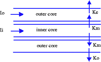

  

  Longitudinal currents.

• I _i (z,t) is the total longitudinal current flowing in the +z direction in the inner conductor measured in amps.

The Core Conductor Model is built on the following assumptions:

• 1. The cell membrane is a cylindrical boundary separating two conductors of current called the intracellular and extracellular solutions. We assume these solutions are homogeneous, isotropic and obey Ohm’s Law.

• 2. All electrical variables have cylindrical symmetry.

• 3. A circuit theory description of currents and voltages is adequate for our model.

• 4. Inner and outer currents are axial or longitudinal only. Membrane currents are radial only.

• 5. At any given position longitudinally (i.e. along the cylinder) the inner and outer conductors are equipotential. Hence, potential in the inner and outer conductors is constant radially. The only radial potential variation occurs in the membrane.

Finally, we assume the following geometric parameters:

• r ₀ is the resistance per unit length in the outer conductor measured in $\frac {ohm}{cm}$.

• r _i is the resistance per unit length in the inner conductor measured in $\frac {ohm}{cm}$.

• a is the radius of the inner cylinder measured in cm.

It is also convenient to define the current per unit area variable J _m : J _m (z,t) is the membrane current density per unit area measured in $\frac {amp}{cm^{2}}$.

Building the core conductor model

Now let’s look at a slice of the model between positions z and z + Δ z. In Figure 5, we see an abstraction of this. The vertical lines represent the circular cross sections through the cable at the positions z and z+Δ z. We cut through the outer shell first giving two horizontal lines labeled outer membrane at the bottom of the figure. Then as we move upward, we encounter the outer conductor. We then move through the inner cable which has a bottom membrane, an inner conductor and a top membrane. Finally, we enter the outer conductor again and exit through the outer membrane. At each position z, there are values of I _i , I _o , V _i , V _o , K _m and V _m that are shown. Between z and z+Δ z, we thus have a cylinder of inner and outer cable of length Δ z. From the Δ z slice in Figure 5, we can abstract an electrical network model and using the standard Kirchoff laws of voltage and current balance at the relevant nodes, we find

$$\begin{array}{@{}rcl@{}} & &\frac{I_{i}(z^{*},t) - I_{i}(z,t)}{\Delta z} = -K_{m}(z,t), \quad \frac{I_{o}(z^{*},t) - I_{o}(z,t)}{\Delta z} \\&&\hspace*{71pt}= K_{m}(z,t) - K_{e}(z,t)\\ & &\frac{V_{i}(z^{*},t) - V_{i}(z,t)}{\Delta z} = -r_{i} I_{i}(z^{*},t), \quad \frac{V_{o}(z^{*},t) - V_{o}(z,t)}{\Delta z}\\ &&\hspace*{78pt}= -r_{o} I_{o}(z^{*} z,t) \end{array} $$

Figure 5

The two slice model.

where to save space we have let z ^∗ denote z+Δ z. Now the equations above apply for any choice of Δ z. Physically, we expect the voltages and currents we see here to be smooth differentiable functions of z and t. Hence, we expect that if we let Δ z go to zero, we will obtain the Core equations: we have V _m =V _i − V ₀ and

$$\begin{array}{*{20}l} \frac{\partial I_{i}}{\partial z} &= -K_{m}(z,t), \quad \quad \frac{\partial I_{o}}{\partial z}= K_{m}(z,t) - K_{e}(z,t) \end{array} $$

((8))

$$\begin{array}{*{20}l} \frac{\partial V_{i}}{\partial z} &= -r_{i} I_{i}(z,t), \quad \quad \frac{\partial V_{o}}{\partial z} = -r_{o} I_{o}(z,t) \end{array} $$

((9))

Note Equation 9 implies that $\frac {\partial V_{m}}{\partial z} = \frac {\partial V_{i}}{\partial z} \: - \: \frac {\partial V_{0}}{\partial z}$. Then, again from Equation 9, we have $\frac {\partial V_{m}}{\partial z} = -r_{i} I_{i} \: + \: r_{o} I_{o}$ Thus, using Equation 8, we obtain

$$\frac{\partial^{2} V_{m}}{\partial z^{2}} =-r_{i} \frac{\partial I_{i}}{\partial z} \: + \: r_{o} \frac{\partial I_{0}}{\partial z} = r_{i} K_{m} \: + \: r_{o} K_{m} \: - \: r_{o} K_{e} $$

Thus, the core equations imply that the membrane voltage satisfies the Core Conductor Equation

$$ \frac{\partial^{2} V_{m}}{\partial z^{2}} =(r_{i} \: + \: r_{o}) K_{m} \: - \: r_{o} K_{e} $$

((10))

The transient cable equations

Normally, we find it useful to model stuff that is happening in terms of how far things deviate or move away from what are called nominal values. We can use this idea to derive a new form of the Core Conductor Equation which we will call the Transient Cable Equation. Let’s denote the rest values of voltage and current in our model by adding a superscript 0 to all of the relevant variables: i.e. ${V_{m}^{0}}$ is the rest value of the membrane potential, ${K_{m}^{0}}$ is the rest value of the membrane current per length density and so forth. It is then traditional to define the transient variables as perturbations from these rest values using the same variables but with lower case letters:

• $v_{m} = V_{m}(z,t) \: - \: {V_{m}^{0}}$ is the deviation of the membrane potential from rest.

• $i_{i} = I_{i}(z,t) \: - \: {I_{i}^{0}}$ is the deviation of the current in the inner fluid from rest.

• $i_{o} = I_{o}(z,t) \: - \: {I_{o}^{0}}$ is the deviation of the current in the outer fluid from rest.

• $v_{i} = V_{i}(z,t) \: - \: {V_{i}^{0}}$ is the deviation of the voltage in the inner fluid from rest.

• $v_{o} = V_{o}(z,t) \: - \: {V_{o}^{0}}$ is the deviation of the voltage in the outer fluid from rest.

• $k_{m} = K_{m}(z,t) \: - \: {K_{m}^{0}}$ is the deviation of the membrane current density from rest.

Then, the core conductor equation in terms of transient variables the Transient Cable Equation or just Cable Equation

$$ \frac{\partial^{2} v_{m}}{\partial z^{2}} \: - \: (r_{i} \: + \: r_{o}) c_{m} \frac{\partial v_{m}}{\partial t} \: - \: (r_{i} \: + \: r_{o}) g_{m} v_{m} = -r_{o} k_{e} $$

((11))

The Cable Equation 11 can be further rewritten in terms of two new constants, the space constant of the cable, λ _c and the time constant, τ _m . Note, we can rewrite 11 as

$$\frac{1}{(r_{i} \: + \: r_{o})g_{m}} \frac{\partial^{2} v_{m}}{\partial z^{2}} \: - \: \frac{c_{m}}{g_{m}} \frac{\partial v_{m}}{\partial t} \: - \: v_{m} = -\frac{r_{o}}{(r_{i} \: + \: r_{o})g_{m}} k_{e} $$

Define the new constants

$$\lambda_{c} = \sqrt{\frac{1}{(r_{i} \: + \: r_{o})g_{m}}} \quad \text{and} \quad \tau_{m} = \frac{c_{m}}{g_{m}} $$

Then $\frac {r_{o}}{(r_{i} \: + \: r_{o})g_{m}} = r_{o} \: {\lambda _{c}^{2}}$ and the Cable Equation 11 can be written in a new form as

$$ {\lambda_{c}^{2}} \: \frac{\partial^{2} v_{m}}{\partial z^{2}} \: - \: \tau_{m} \: \frac{\partial v_{m}}{\partial t} \: - \: v_{m} = -r_{o} {\lambda_{c}^{2}} \: k_{e} $$

((12))

The new constants τ _m and λ _c are very important to understanding how the solutions to this equation will behave. We call τ _m the time constant and λ _c the space constant of our cable. To understand the Time Constant, consider the ratio $\frac {c_{m}}{g_{m}}$. Note the ratio has units of seconds and thus, we can interpret this constant as the time constant of the cable, τ _m . Note that τ _m is a constant whose value is independent of the size of the cell; hence it is a membrane property. We can show the time constant can thus be expressed as $\frac {c_{m}}{g_{m}}$ also. Next consider the Space Constant. Look at the dimensional analysis of the term $\frac {1}{(r_{i}+r_{o}) g_{m}}$ which has units of cm ². This is why the square root of the ratio functions as a length parameter. We can look at this more closely. Consider again our approximate model where we divide the cable up into pieces of length Δ z. If we do some standard biophysical analysis, we can show $\lambda _{c} = \sqrt {\frac {a}{2 \rho _{i} G_{m}}}$. Now ρ _i and G _m are membrane constants independent of cell geometry. So we see that the space constant is proportional to the square root of the fiber radius. Note also that the space constant decreases as the fiber radius shrinks.

Finite cables

We are actually interested in a model of information processing that includes a finite length dendrite, a cell body and an axon. Consider a family of problems of the form (13)

((13))

where is the conductance to the end cap at position L and the family $\left \{{k_{e}^{c}}\right \}$ of impulses are each zero off [z ₀−C, z ₀+C], symmetric around z ₀ and the area under the curve is 1 for all C. So the pulse family always delivers a constant 1 amp of current and we control the magnitude of the delivered current by the multiplier I ₀. We assume for now that the site of current injection is z ₀ which is in (0,L). As C goes to 0 in the solutions of this model, we obtain the limiting solution

$$v_{m}(z) = \frac{r_{0} \lambda_{c} I_{0}}{2} e^{-\frac{|z-z_{0}|}{\lambda_{c}}}, \: \: 0 \: \leq \: z \: \leq \: L $$

which is the idealized impulse solution to the infinite cable model.

The ball and stick model

We now extend our simple dendritic cable model to what is called the ball and stick neuron model. This consists of an isopotential sphere to model the cell body or soma coupled to a single dendritic fiber input line. We model the soma as a simple parallel resistance/capacitance network and the dendrite as a finite length cable as previously discussed (see Figure 6). In Figure 6, you see the terms I ₀, the input current at the soma/dendrite junction starting at τ=0;I _D , the portion of the input current that enters the dendrite (effectively determined by the input conductance to the finite cable, G _D ); I _S , the portion of the input current that enters the soma (effectively determined by the soma conductance G _S ); and C _S , the soma membrane capacitance. We assume that the electrical properties of the soma and dendrite membrane are the same; this implies that the fundamental time and space constants of the soma and dendrite are given by the same constant (we will use our standard notation τ _M and λ _C as usual). For convenience, we now normalized the variables using the transformations

$$\tau = \frac{t}{\tau_{M}}, \: \: \lambda = \frac{z}{\lambda_{C}}, \: \: L = \frac{\ell}{\lambda_{C}}, \: \: \Longrightarrow \hat{v}_{m} = v_{m}(\lambda_{C} \lambda,\tau_{M} \tau). $$

It is then possible to show that with a reasonable zero-rate left end cap condition the appropriate boundary condition at λ=0 is given by

$$ \rho \: \frac{\partial \hat{v}_{m}}{\partial \lambda}(0,\tau) = \tanh(L)\left[\hat{v}_{m}(0,\tau) \: + \: \frac{\partial \hat{v}_{m}}{\partial \tau}(0,\tau) \right], $$

((14))

Figure 6

The ball and stick model.

where we introduce the fundamental ratio $\rho = \frac {G_{D}}{G_{S}}$, the ratio of the dendritic conductance to soma conductance (Rall 1977). The full system to solve is therefore:

$$\begin{array}{*{20}l} \frac{\partial^{2} {\hat{v}_{m}} }{\partial {\lambda^{2}} } &= \hat{v}_{m} + \frac{\partial {\hat{v}_{m}}}{\partial \tau}, \: \: 0 \: \leq \lambda \: \leq \: L, \: \: \tau \: \geq \: 0. \end{array} $$

((15))

$$\begin{array}{*{20}l} \frac{\partial \hat{v}_{m}}{\partial \lambda}(L,\tau) &= 0, \quad \rho \: \frac{\partial \hat{v}_{m}}{\partial \lambda}(0,\tau) = \tanh(L) \left[ {\vphantom{\frac{0}{0}}}\hat{v}_{m}(0,\tau) \: \right.\\&\quad \left.+\quad \: \frac{\partial \hat{v}_{m}}{\partial \tau}(0,\tau) \right]. \end{array} $$

((16))

Applying the technique of separation of variables, $\hat {v}_{m}(\lambda, \tau) \: = \: u(\lambda) w(\tau)$, we find there are is infinite family of solutions $\hat {v}_{m}^{n}(\lambda,\tau) = A_{n} \: \cos (\alpha _{n} \lambda) \: e^{- \left (1 + {\alpha _{n}^{2}}\right) \tau }$ where the values α _n satisfy the transcendental equation

$$ \tan(\alpha L) = - \alpha \: \frac{\tanh(L)}{\rho} \: = \: - \kappa(\alpha L), $$

((17))

where $\kappa = \frac {\tanh (L)}{\rho L}$. This is not a traditional Fourier series solution but we can show the general solution has the form

$$\hat{v}_{m}(\lambda,\tau)= A_{0} \: e^{-\tau} \: + \: \sum\limits_{n=1}^{\infty} \: A_{n} \: \cos(\alpha_{n} (L - \lambda)) e^{-\left(1 + {\alpha_{n}^{2}}\right) \tau}. $$

To solve this model, for an applied continuous voltage pulse V applied to the cable, we expand V as

$$V(\lambda) = V_{0} \: + \: \sum\limits_{n=1}^{\infty} \: V_{n} \: \cos(\alpha_{n} (L - \lambda)) $$

and match coefficients from the expansion of $\hat {v}_{m}(\lambda,0)$. We can show any voltage pulse of interest can be written this way (Peterson J, BioInformation Processing: A Primer on Computational Cognitive Science in the Springer Cognitive Science and Technology Series, in press). Thus, an approximate solution is given by

$$ \hat{v}_{m}(\lambda,\tau) \approx A_{0} \: e^{-\tau} + \sum\limits_{n=1}^{Q} \: A_{n} \: \cos(\alpha_{n} (L - \lambda)) \: e^{-(1 + {\alpha_{n}^{2}}) \tau} $$

((18))

The calculation of the first Q coefficients is then handled as a linear algebra problem.

We can also solve the full time and space cable equation using a different suite of mathematical tools. We convert the cable equation

$${\lambda_{c}^{2}} \: \frac{\partial^{2} v_{m}}{\partial z^{2}} = v_{m} \: + \: \tau_{m} \: \frac{\partial v_{m}}{\partial t} \: - \: r_{o} \: {\lambda_{c}^{2}} \: k_{e}, $$

where k _e is current pulse per unit length applied at one point into a diffusion equation with a change of variables. First, we introduce a dimensionless scaling to make it easier via the change of variables: $y \: = \: \frac {z}{\lambda _{c}}$ and $s \: = \: \frac {t}{\tau _{m}}$. With these changes, space will be measured in units of space constants and time in units of time constants. We then define the a new voltage variable w by w(s,y)=v _m (τ _m t,λ _c z) giving us the scaled cable equation $\frac {\partial ^{2} w}{\partial y^{2}} = w \: + \: \frac {\partial w}{\partial s} \: - \: r_{o} \: {\lambda _{c}^{2}} \: k_{e}(\tau _{m} s, \lambda _{c} y)$. Then make the additional change of variables Φ(s,y)=w(s,y) e ^s and obtain the new model

$$ \frac{\partial^{2} \Phi}{\partial y^{2}} =\frac{\partial \Phi}{\partial s} \: - \: r_{0} {\lambda_{c}^{2}} \: \tau_{m} \: k_{e}(\tau_{m} s, \lambda_{c} y) \: e^{s}. $$

((19))

We go back to thinking of the cable as a half infinite one to simplify the ideas and apply both the Laplace and Fourier transform to this model to solve in the transformed variables. We then invert to find a time dependent solution to this cable model

$$\Phi(s,y) = r_{0} \lambda_{c} I_{0} \: \frac{1}{\sqrt{4 \pi s}} \: e^{- \frac{y^{2}}{4s}} $$

Note, if we think of the diffusion constant as $D_{0} = \frac {{\lambda _{c}^{2}}}{\tau _{m}}$, we can rewrite Φ(s,y) as follows:

$$\Phi(s,y) = r_{0} {\lambda_{c}^{2}} I_{0} \: \frac{1}{\sqrt{4 \pi D_{0} t}} \: e^{- \frac{x^{2}}{4 D_{0} t }} $$

Note the term $P_{0}(x,t) = \frac {1}{\sqrt {4 \pi D_{0} t}} \: e^{- \frac {x^{2}}{4 D_{0} t }}$ is the usual probability density function for a random walk with space constant $\lambda _{c}/\sqrt {2}$ and time constant τ _m . Thus, Φ(s,y)=(r ₀ λ _c )I ₀ (λ _c P ₀(x,t)). The term λ _c P ₀(x,t) is the probability we are in an interval of width λ _c /2 around x and so is a scalar without units. We then find the full solution w

$$w(s,y) = \Phi(s,y) \: e^{-s} = r_{0} \lambda_{c} I_{0} \: \frac{1}{\sqrt{4 \pi s}} \: e^{- \frac{y^{2}}{4s}} \: e^{-s}. $$

We write this in the unscaled form at the pulse center (t ₀,z ₀) as

$$ v_{m}(t,z) = r_{0} \lambda_{c} I_{0} \: \frac{1}{\sqrt{4 \pi \: ((t-t_{0})/\tau_{m})}} \: e^{- \frac{((z-z_{0})/\lambda_{c})^{2}} {4 ((t-t_{0})/\tau_{m}) }} \: e^{-(t-t_{0})/\tau_{m})} $$

((20))

Note the differences between the solution we find by using separation of variables techniques where we assume the time and spatial parts of the solution are separated which forces us to use an infinite series approach. This also introduces numerical artifacts and so forth. The solution using transform tools shows a very different time and space dependence in the solution which means the decay of the response to the voltage impulse applied to the cable is actually different than a standard exponential decay. Still, a nice guiding principle is that the response drops roughly e ⁻¹ in magnitude every time and space constant we move away from the injection site. Also, please note that we make a large number of simplifying assumptions in order to arrive at these results.

The basic Hodgkin - Huxley model

We now discuss the Hodgkin - Huxley model for the generation of the action potential of an excitable nerve cell using the standard Ball and Stick model. This augmented cable equation can also be solved using the transform techniques but we will not do so here. As previously mentioned, there are many variables are needed to describe what is happening inside and outside the cellular membrane, and to some extent, inside the membrane for a standard cable model. In the standard core conductor model, the membrane is not modeled at all, but we now need to be more careful. A realistic description of how the membrane activity contributes to the membrane voltage must use models of ion flow which are controlled by gates in the membrane. A simple model of this sort is based on work that Hodgkin and Huxley ((Hodgkin and Huxley 1952), (Hodgkin 1952), (Hodgkin 1954)) performed in the 1950’s. We start by expanding the membrane model to handle potassium, sodium and an all purpose current, called leakage current, using a modification of our original simple electrical circuit model of the membrane. We will think of a gate in the membrane as having an intrinsic resistance and the cell membrane itself as having an intrinsic capacitance as shown in Figure 7. This is a picture of an idealized cell with a small portion of the membrane blown up into an idealized circuit: we see a small piece of the lipid membrane with an inserted gate. Thus, we expand the single branch of our old circuit model to multiple branches – one for each ion flow we wish to model. The ionic current consists of the portions due to potassium, K _K , sodium, K _Na and leakage K _L . The leakage current is due to all other sources of ion flow across the membrane which are not being explicitly modeled. This would include ion pumps; gates for other ions such as Calcium, Chlorine; neurotransmitter activated gates and so forth. We will assume that the leakage current is chosen so that there is no excitable neural activity at equilibrium. We know that conductance is reciprocal resistance, so our model will consist to a two branch circuit: one branch is contains a capacitor and the other, the conductance element. We will let c _m denote the membrane capacitance density per unit length (measured in $\frac {fahrad}{cm}$). Hence, in our membrane box which is Δ z wide, we see the value of capacitance should be c _m Δ z. Similarly, we let g _m be the conductance per unit length (measured in $\frac {1}{ohm-cm}$) for the membrane. The amount of conductance for the box element is thus g _m Δ z. In Figure 8, we illustrate our new membrane model. Since this is a resistance - capacitance parallel circuit, it is traditional to call this an RC membrane model. In Figure 8, the current going into the element is K _m (z,t)Δ z and we draw the rest voltage for the membrane as a battery of value ${V_{m}^{0}}$. We know thatthe membrane current, K _m , satisfies Equation 21:

$$ K_{m}(z,t) = g_{m} \: V_{m}(z,t) \: + \: c_{m} \frac{\partial V_{m}}{\partial t} $$

((21))

Figure 7

The membrane and gate circuit model.

Figure 8

The RC membrane model.

In terms of membrane current densities, all of the above details come from modeling the simple equation K _m =K _c + K _ion where K _m is the membrane current density, K _c is the current through the capacitative side of the circuit and K _ion is the current that flows through the side of the circuit that is modeled by the conductance term, g _m . We see that in this model $K_{c} = c_{m} \frac {\partial V_{m}}{\partial t}$ and K _ion =g _m V _m . However, we can come up with a more realistic model of how the membrane activity contributes to the membrane voltage by adding models of ion flow controlled by gates in the membrane. Our models are based on work that Hodgkin and Huxley performed in the 1950’s.

The standard Hodgkin - Huxley model of an excitatory neuron consists of the equation for the total membrane current, K _M , obtained from Ohm’s law: $K_{m} = c_{m} \frac {\partial V_{m}}{\partial t} \: + \: K_{K} \: + \: K_{\textit {Na}} \: + \: K_{L}$ where we have expanded the K _ion term to include the contributions from the sodium and potassium currents and the leakage current. The new equation for the membrane voltage is thus

$$\begin{array}{@{}rcl@{}} \frac{1}{r_{i} \: + \: r_{o}} \: \frac{\partial^{2} V_{m}}{\partial z^{2}} &=& c_{m} \frac{\partial V_{m}}{\partial t} \: + \: K_{K} \: + \: K_{Na} \: + \: K_{L} \:\\ &&- \: \frac{r_{o}}{r_{i} \: + \: r_{o}} \: K_{e} \end{array} $$

((22))

In Figure 1, we show an idealized cell with a small portion of the membrane blown up into an idealized circuit. We see a small piece of the lipid membrane with an inserted gate. We think of the gate as having some intrinsic resistance and capacitance. Now for our simple Hodgkin - Huxley model here, we want to model a sodium and potassium gate as well as the cell capacitance. So we will have a resistance for both the sodium and potassium. In addition, we will have additional ion currents modeled as a leakage current with its own resistance. We also know that each ion has its own equilibrium potential which is determined by applying the Nernst equation. The driving electromotive force or driving emf is the difference between the ion equilibrium potential and the voltage across the membrane itself. Hence, if E _c is the equilibrium potential due to ion c and V _m is the membrane potential, the driving force is V _c − V _m . Looking back again, Figure 1, we see an electric schematic that summarizes what we have just said. We model the membrane as a parallel circuit with a branch for the sodium and potassium ion, a branch for the leakage current and a branch for the membrane capacitance. As usual, from Ohm’s law, we know for each ion $c, I_{c} = \frac {1}{R_{c}} \: V_{c}$ or I _c =G _c V _c where G _c is the reciprocal resistance or conductance of ion c. Hence, we can model all of our ionic currents using a conductance equation of the form above. Of course, the potassium and sodium conductances are nonlinear functions of the membrane voltage V and time t. This reflects the fact that the amount of current that flows through the membrane for these ions is dependent on the voltage differential across the membrane which in turn is also time dependent. The general functional form for an ion c is thus I _c =G _c (V,t)(V(t)−E _c (t)) where as we mentioned previously, the driving force, V−E _c , is the difference between the voltage across the membrane and the equilibrium value for the ion in question, E _c . Note, the ion battery voltage E _c itself might also change in time (for example, extracellular potassium concentration changes over time). Hence, the driving force is time dependent. The conductance is modeled as the product of an activation, m, and an inactivation, h, term and it is assumed to have the form G _c (V,t)=G ₀ m ^p(V,t) h ^q(V,t) where appropriate powers of p and q are found to match known data for a given ion conductance. Finally, we model the leakage current, I _L , as I _L =g _L (V(t)−E _L ) where the leakage battery voltage, E _L , and the conductance g _L are constants that are data driven. Hence, in terms of current densities, letting g _K ,g _Na and g _L respectively denote the ion conductances per length, our full model would be

$$\begin{aligned} \frac{1}{r_{i} + r_{o}} \frac{\partial^{2} V_{m}}{\partial z^{2}} &= c_{m} \frac{\partial V_{m}}{\partial t} \: + g_{K} \left(\Delta {V_{m}^{K}}\right) + g_{Na} \left(V_{m}^{Na}\right) \\&+ g_{L} \left({V_{m}^{L}}\right) - \frac{r_{o}}{r_{i} + r_{o}} K_{e} \end{aligned} $$

where we have written $\Delta {V_{m}^{K}} = V_{m} - E_{K}$ and so forth. Under certain experimental conditions, we can force the membrane voltage to be independent of the spacial variable z. In this case, we find $\frac {\partial ^{2} V_{m}}{\partial z^{2}} = 0$ which allows us to write

$$ c_{m} \frac{d V_{m}}{d t} \: + \: K_{K} \: + \: K_{Na} \: + \: K_{L} \: - \: \frac{r_{o}}{r_{i} \: + \: r_{o}} \: K_{e} = 0 $$

((23))

Since, c _m is capacitance per unit length, the above equation can also be interpreted in terms of capacitance, C _m , and currents, I _K , I _Na , I _L and an external type current I _e . This leads to

$$ C_{m} \frac{d V_{m}}{d t} \: + \: I_{K} \: + \: I_{Na} \: + \: I_{L} \: - \: \frac{r_{o}}{r_{i} \: + \: r_{o}} \: I_{e} = 0 $$

((24))

Finally, if we label as external current, I _e , the term $I_{E} = \frac {r_{o}}{r_{i} \: + \: r_{o}} \: I_{e}$, the equation we need to solve under the voltage clamped protocol becomes

$$ \frac{d V_{m}}{d t} = \frac{1}{C_{M}} \left (- \: I_{K} \: - \: I_{Na} \: - \: I_{L} \: + \: I_{E} \right) $$

((25))

The Hodgkin-Huxley sodium and potassium model

Hodgkin and Huxley modeled the sodium and potassium gates as

where and are called activation variables and is an inactivation variable which all satisfy the first order Φ kinetics that tell us

where for each ion c

Further, the coefficient functions, α and β for each variable required data fits, such as , as functions of voltage. We will not list the rest here as we do not need that level of detail. Of course these data fits were obtained at a certain temperature and assumed values for all the other constants needed and so they need to be altered if the temperature and ionic concentrations change. Our model of the membrane dynamics here thus consists of the following differential equations:

We note that at equilibrium there is no current across the membrane. Hence, the sodium and potassium currents are zero and the activation and inactivation variables should achieve their steady state values which would be m _∞ , h _∞ and n _∞ computed at the equilibrium membrane potential which is here denoted by V ₀.

At this point, we see a general model of how to generate an action potential. We do not model the transmission of the action potential to its target neurons; suffice it to say, there are molecular mechanisms that send the pulse to its targets without change. At the interface to the target neuron called the synapse, the incoming voltage pulse generates a Ca ⁺² current which in turn generates discrete packets of neurotransmitter which are released for processing by the target neurons dendritic subsystem. Note the signal transduction pathway here: the axonal voltage pulse is converted into a discrete release of molecules which bind with the dendritic arbor and thereby shape the next axonal pulse in very nonlinear ways. We are also not interested here in how information might be encoded in collections of axonal spikes. Our interest at the moment is in the low level bones. In general, we separate the effects of these triggers into two classes: first messengers which are essentially voltage activated gates and second messengers which enter through the membrane and initiate a protein transcription event which can rebuild the actual hardware of the cell. An abstract analysis of such a trigger event is presented in (Peterson 2014a) in order to build trigger approximations. Here, we will primarily be interested in second messengers which are neurotransmitters even though the triggers can be more general. There is a vast literature on signaling in a biological neural system and we will point you to just a few relevant sources. We prefer papers and texts that help us understand an overarching theory of the signaling process. Most of these sources are actually fairly old but are full of the technical detail needed to understand the processes being studied. In particular, the use of mathematical points of view is not shied away from and newer references tend to downplay that point of view. Two basic and very useful texts on signaling are (Gerhart and Kirschner 1997) and (Wilkins 2002) which look at these ideas very theoretically. Two other very good resources for this material are (Hille 1992) and (Bray 1998). Bray’s paper is very important and is very useful when you try to understand signaling principles; again, the material is not really dated and it is worth a strong push towards assimilating its ideas. Remember that understanding signaling principles allows us to see how to build reasonable approximations. The paper (Sneppen et al. 2010) is really about protein networks but it has lots of good advice about how to approximate complicated biophysics and then glue together the models into systems. A good overview of how neurons work together to generate high level behavior (which we do not really understand) can be found in (Roberts et al. 2010) which will help you see Black’s points discussed in the next section again phrased in terms of what we currently understand. There is a lot of combinatorial complexity here too and modeling that is hard. Even 4 things taken 2 at a time at each node leads to incredible explosions of computation. A really interesting article on dealing with that is found in (Borisov et al. 2006) which is well worth a read. Another look at the notion of discrete synaptic states and resulting computational complexity is in (Montgomery and Madison 2004) and (Harris-Warrick and Johnson 2010). With all this said, for simplicity, let’s look now at the class of catecholamine neurotransmitters in the nervous system. We will focus on only a few types: DA, dopamine; NE, norepinephrine; and E, epinephrine and lump them together into the category called CAs because they all share a common core biochemical structure, the catechol group.

Modeling issues

Consider the following perceptive quotation (Black 1991):

“More generally, regulation of transmitter synthesis shares important commonalities in neurons that differ functionally, anatomically, and embryologically. This point is worthy of emphasis. Simply stated, the common biochemical and genomic organization of these diverse populations determines how environmental, epigenetic information, through altered impulse activity, is translated into neural information... cellular biochemical organization, not behavioral modality, is a key determinant of how external stimuli are converted into neural language. In this domain, modes of information storage are biochemically specific, not modality specific, indicating that synaptic systems subserving entirely different behavioral and cognitive functions may share common modes of information processing (boldface our choice)”

Hence, in our search for a core object useful in constructing architectures capable of subserving learning and memory function among other things, the evidence above suggests we focus on various second messengers such as prototypical neurotransmitters. Figure 3 indicates to us that the general structure of a typical action potential contains some important points we can organize into a low dimensional feature vector

$$\xi = \,[(t_{0}, V_{0}), (t_{1}, V_{1}),(t_{2}, V_{2}), (t_{3}, V_{3}),(g, t_{4}, V_{4})]^{\prime} $$

where (t ₀,V ₀) is the start point of the pulse, (t ₁,V ₁) is where the maximum occurs, (t ₂,V ₂) is when the voltage returns to reference voltage, (t ₃,V ₃) is the location of the minimum and the model of the tail of the action potential during the bulk of hyperpolarization phase has the form V _m (t)=V ₃ + (V ₄−V ₃) tanh(g(t−t ₃)). Hence, from a certain point of view, these 11 parameters capture much of the important information about this pulse. Second messengers are triggers which enter the dendrite, soma and/or axon and initiate the transcription of one or multiple proteins. Since these proteins include those used to build sodium and potassium gates, we see a second messenger trigger can influence directly $g^{Max}_{\textit {Na}}$ and $g^{Max}_{K}$ and thereby reshape the pulse. In general, a neurotransmitter can initiate a change in the shape of the action potential which we can for simplicity corresponds to an alteration of the 11 parameters that shape the feature vector. Hence, a trigger T generates δ ξ=[(δ t ₀,δ V ₀),(δ t ₁,δ V ₁),(δ t ₂,δ V ₂),(δ t ₃,δ V ₃),(δ g,δ t ₄,δ V ₄)]^′. Some neurotransmitters can generate an update signal which alters only one parameter and leaves the others alone. Such triggers are quite useful and are used in synthetic biology as orthogonal primers as they allow us to modify one thing at a time, so to speak (Ansari and Mapp 2002), (Esvelt et al. 2013) and (Rusk 2014), but that is another story. Hence, a model of dendritic–axonal interaction should include a mechanism for dendrite and axon object interaction which in general requires an agent which accepts dendritic and axonal arguments. Further, both the dendrite and the axon should have some dependency on neurotransmitters inputs whose construction and subsequent reabsorption for further reuse should follow modulatory pathways that mimic in principle the realities of CA transmitter synthesis.

How should we model CA release, CA termination, CA identification via CA specific receptors and synaptic plasticity? CA is released through a large variety of mechanisms, each of which is modulated in varying degrees by many other agents. Most importantly, this release needs C a ⁺² which is mediated by second messenger action such hormones and intraneural cAMP in what can be a rather global way. Hence, release of CA itself can modulate subsequent CA release. Further, there are more global mechanisms which interact with the CA release and production cycle via non–transmitter mechanisms. Note (Black 1991)

“...angiotensin II receptors on the [presynaptic] membrane also modulate norepinephrine release. Angiotensin is a potent vasoconstrictor, derived from... an enzyme secreted by the kidney...the principle is startling: the kidney can communicate with sympathetic neurons through nonsynaptic mechanisms (boldface choice ours)...Circulating hormone regulates transmitter release at the synapse. Synaptic communication, then, may be modulated by nonsynaptic mechanisms, and distant structures may talk to receptive neurons. Consequently aspects of communication with the nervous system are freed from hard–wiring constraints (boldface choice author’s).”

Clearly, dendritic–axonal software interaction should be mediated via pathways of both local scope objects) and global scope, using additional objects which could be modeled after hormones.

We also know CA termination is critical to CA function. CA substance is deactivated by reabsorption into the presynaptic structure itself. For example, dopamine levels are controlled by three separate mechanisms.

• Dopamine packets are released into the synaptic cleft and bind to receptors on the dendrite. So, the number of receptors per unit area of dendritic membrane provides a control of dopamine concentration in the cleft.

• Dopamine is broken down by enzymes in the cleft all the time which also control dopamine concentration.

• Dopamine is pumped back into the presynaptic bulb for reuse providing another mechanism.

Hence, the interaction between the presynaptic and postsynaptic neurons is always changing. This mutability is called their synaptic plasticity. It is mediated by both local and global pathways. Indeed, it is clear an attempt to develop a large scale architecture which possesses sufficient plasticity will be a daunting task. We must remember (Black 1991)

“Briefly, certain types of molecules in the nervous system occupy a unique functional niche. These molecules subserve multiple functions simultaneously.... [They] incorporate environmental information into the cell and nervous system. Consequently these molecules simultaneously function as biochemical intermediates and as symbols representing specific environmental conditions.... The principle of multiple function implies that there is no clear distinction among the processes of cellular metabolism, intercellular communication, and symbolic function in the nervous system. Representation of information and communication are part of the functioning fabric of the nervous system.... the brain can no longer be regarded as the hardware underlying the separate software of the mind. Scrutiny will indicate that these categories are ill framed and that hardware and software are one in the nervous system.”

From this quote of Black, you can see the enormous challenge we face. We can infer from the above that to be able to have the properties of plasticity and response to environmental change, certain software objects in our model must be allowed to subserve the dual roles of communication and architecture modification. Black refers to this as the “principle of polyfunction” (Black 1991).

“Shorn of all detail, the software–hardware dichotomy is artificial.... software and hardware are one and the same in the nervous system. To the degree that these terms have any meaning in the nervous system, software changes the hardware upon which the software is based. For example, experience changes the structure of neurons, changes the signals that neurons send, changes the circuitry of the brain, and thereby changes output and any analogue of neural software.”

How are we to design a software architecture system which essentially is self–modifying? Next, note (Black 1991)

“Increasing evidence indicates that ongoing function, that is, communication itself, alters the structure of the nervous system. In turn altered structure changes ongoing function, which continues to alter structure. The essential unity of structure and function is a major theme...... In this system, then, signal communication, growth, altered architecture, altered neural function, and memory are causally interrelated; there is no easy divide between hardware and software. The rules of function are the rules of architecture, and function governs architecture, which governs function.... The essential unity of structure and function, of hardware and software, is not restricted to mammals; it is evident in invertebrate nervous systems as well.”

If we think of architectures consisting of loosely coupled computational modules, each module is a kind of input–output mapping which we can call an object of type IOMAP. Models with computational nodes linked by edges can be called graph models. Early versions of these software architectures for neural systems assert the information content of the architecture is stored in the weight values are attached to the links and these weight values are altered due to environmental influence via some sort of updating mechanism. Since it is now clear the architecture itself must be self–modifying, consider the dual roles played by neural processing elements (Black 1991):

“Any set of elements is relevant only insofar as it processes information and simultaneously participates in ongoing neural function; these dual roles require the neural context. What structural elements may be usefully examined?... First, neural elements of interest must change with environment. That is, environmental stimuli must, in some sense, regulate the function of these particular units such that the units actually serve to represent conditions of the real world. The potential units, or elements of interest, thereby function as symbols representing external or internal reality. The symbols, then, are actual physical structures that constitute neural language representing the real world (boldface our choice). Second, the symbols must govern the function of the nervous system such that the representation itself constitutes a change in neural state. Consequently symbols do not serve as indifferent repositories of information but govern ongoing function of the nervous system (boldface our choice). Symbols in the nervous system simultaneously dictate the rules of operation of the system.... The syntax of symbol operation is the syntax of neural function (boldface our choice).”

Vertebrates use this sort of grammar building in many situations. It is very interesting to compare these neural ideas to similar ideas in immunology (see (Shastri et al. 2002), (Rot and von Andrian 2004) and (Edwards et al. 2012)); compare the grammars implicitly encoded by chemokine signals to what are encoded by neural signals. Indeed inflammatory responses due to cytokine grammar parsing are probably responsible for some psychopathology (Capuron and Miller 2004). Information processing also involves a combinatorial strategies (Black 1991):

“Two related strategies are employed by the nervous system in the manipulation of the transmitter molecular symbols. First, individual neurons use multiple transmitter signal types at any given time. Second, each transmitter type may respond independently of others to environmental stimuli.... The neuron appears to use a combinatorial strategy, a simple and elegant process used repeatedly in nature in a variety of guises. A series of distinct elements, of relatively restricted number, are used in a wide variety of combinations and permutations.”

In our mind, although there is an architecture that specifies connection information between processing nodes, what really counts is how the computation is organized into overlapping computational modules. It is dangerous to think that these neural systems are organized hierarchically. In (Wagner 2014), there is a compelling discussion of hierarchical schemes which is targeted towards problems in homology, the study of how characteristics in different species are similar and could even have evolved from a common ancestor. Wagner says it best:

“We have to emancipate our thinking from the hierarchical concept of how bodies of organisms are organized. In fact, hierarchy never made sense if one thinks of the body as an integrated system that contains differentiated parts. Integration is primary, differentiation is secondary and how the body becomes parceled into modular units does not follow a hierarchical logic (boldface our choice)”

We face very similar conceptual issues in our development of a model of a neural system. We believe the fundamental computational entities of the neural system do organize in time constrained and, perhaps, spatially constrained, collections of nodes and that it is quite simplistic to try to analyze this using modules and hierarchies. Wagner notes, in discussing how cell type is determined

“there is increasing evidence that the gene regulatory network state of a cell is governed not by one core network, but by a mosaic of densely interconnected network modules each of which, in isolation, might look like a core network.”

He goes on further to note that some cell types can be understood as different combinations of gene regulatory modules which is reminiscent of the kind of combinatorial machinations we see in the immune system to generate a response to an intruder ((Shastri et al. 2002) and (Rot and von Andrian 2004)) and in the nervous system ((Black 1991) and (Montgomery and Madison 2004)). Each IOMAP module must therefore be capable of a certain number of active states.

Assembling neurons into networks

The inputs into the dendritic tree of an excitable nerve cell can be separated into first and second messenger classes. The first messenger group consists of Hodgkin-Huxley voltage dependent ion gates and the second messengers includes molecules which bind to the dendrite through some sort of interface and then trigger a series of secondary events inside the cytoplasm of the cell body which lead to protein transcription and the modification of the cell’s molecular machinery. We can connect a standard feedforward architecture of neurons as a chain as shown in Figure 9. Note that in Figure 9, the interaction between dendritic and axonal objects has not been made explicit. The usual simplistic approximation to this interaction transforms a summed collection of weighted inputs via a saturating transfer function with bounded output range. The dendritic and axonal interaction is modeled by a scalar W _ij as described above. It measures the intensity of the interaction between the input neuron i and the output neuron j as a simple scalar weight.

Figure 9

A chained neural architecture with self feedback loops and general feedback.

Chained architecture details

Let’s look at a chain of computational nodes such as neurons in more detail. If the architecture is feed forward we would have the Chain Feed Forward Network (CFFN). The chain consists of computational elements, generally referred to as neurons. This is because a very simple model of neural processing models the action potential spike with a sigmoid function which transitions rapidly from a binary 0 (no spike) to 1 (spike). This sigmoid is called a transfer function and since it can not exceed 1 as 1 is a horizontal asymptote, it is called a saturating transfer function also. This model is known as a lumped sum model of post-synaptic potential; now that we know about the ball - stick model of neural processing, we can see the lumped sum model is indeed simplistic. Each neuron thus processes a summed collection of weighted inputs via a saturating transfer function with bounded output range (i.e. [0,1]). The neurons whose outputs connect to a given target or postsynaptic neuron are called presynaptic neurons. Each presynaptic neuron has an output Y which is modified by the synaptic weight W _{p r e,p o s t} connecting the presynaptic neuron to the postsynaptic neuron. This gives a contribution W _{p r e,p o s t} Y to the input of the postsynaptic neuron. A typical transfer function could be modeled as $\sigma (x,o,g) =.5 \left (1.0 + \tanh \left (\frac {x-o}{\phi (g)} \right) \right)$ where o is the offset which controls the location of the maximum response of the sigmoid and ϕ(g) is a function which shapes how fast the sigmoid rises from its minimum to its maximum value. The chained model then consists of a string of N neurons, labeled from 0 to N−1. Some of these neurons can accept external input and some have their outputs compared to external targets. We let ${\mathcal U} = \text { indices} ~i~ \text {where neuron}~ i~ \text {is an input}$ and ${\mathcal V} = \text {indices} ~i \text { where neuron}~ i~ \text {is an output}$. We will let n _I and n _O denote the size of and respectively. Note in a chain, it is also possible for an input neuron to be an output neuron; hence and need not be disjoint sets. Each neuron can be viewed as a postsynaptic neuron with a set of presynaptic neurons feeding into it: thus, each neuron i has associated with it a set of backward links which will be denoted by (i). Each node i also connects forward to other nodes and the set of forward connections is called ${\mathcal F}(i)$. The weight of the synaptic link connecting the presynaptic neuron i to the postsynaptic neuron j is then denoted by W _i→j although in general this should be an edge processing function. For a feedforward architecture, we would have j > i, however, as you can see in Figure 9, this is not true in more general chain architectures. The input of a typical postsynaptic neuron therefore requires summing over the backward link set of the postsynaptic neuron in the following way:

$$y^{post} = x + \sum\limits_{pre \: \in \: {\mathcal B}(post)} \: W_{pre \rightarrow post} \: Y^{pre} $$

where the term x is the external input term which is only used if the post neuron is an input neuron. The chain thus processes an arbitrary input vector $\boldsymbol {x} \in R^{n_{I}}\phantom {\dot {i}\!}$ into an output vector in $\Re ^{n_{O}}$ and this is a highly nonlinear calculation. In Figure 9, we see a chain of six neurons. We see two neurons that accept external input (neurons 0 and 1) and two neurons having external taps (neurons 4 and 5). The set of postsynaptic neurons for a given neuron i is denoted by the symbols ${\mathcal F}(i)$; the letter denotes the feedforward links, of course. Note the self and feedback connection in the set ${\mathcal F}(2) = \{ 2, 5 \}$. Also each neuron can be viewed as a postsynaptic neuron with a set of presynaptic neurons feeding into it: thus, each neuron i has associated with it a set of backward links which will be denoted by ${\mathcal B}(i)$ such as $\mathcal {B}(5) = \{ 0, 2, 3, 4\}$. In general, the backward link sets can be much richer in connections than this simple example indicates. This model thus uses the computational scheme

$${\fontsize{8.5}{6}\begin{aligned} Y^{post} = \sigma \left(y^{post},o,g \right) \: = \: \sigma \left(x + \sum\limits_{pre \: \in \: {\mathcal B}(post)} \: W_{pre \rightarrow post} \: Y^{pre} \right) \end{aligned}} $$

which can be rewritten $a^{post} = S \left (x + \sum _{pre \in {\mathcal B}(post)} \: a^{pre} \bullet d^{post}, \: p \right)$ where a indicates the value of a given axon, d, the value of a given dendrite and S, the soma computational engine, which depends on a vector of parameters, p. The term a ^pre∙d ^post denotes the interaction or processing between the post neuron axon and the pre neuron dendrite. Note that the ∙ operation could correspond to a simple multiplication of the pre–axon value d and the post–dendrite value d.

Each of our directed graphs also has node and edge functions associated with it and these functions are time dependent as what they do depends on first and second messenger triggers, the hardware structure of the output neuron and so forth. We therefore could model neural circuitry using a directed graph architecture consisting of computational nodes N and edge functions E which mediate the transfer of information between two nodes. Hence, if N _i and N _j are two computational nodes, then E _i→j would be the corresponding edge function that handles information transfer from node N _i and node N _j . For our purposes, we will assume here that the neural circuitry architecture we describe is fixed, although dynamic architectures can be handled as sequence of directed graphs. We then organize the directed graph using interactions between neural modules (visual cortex, thalamus etc) which are themselves subgraphs of the entire circuit. Once we have chosen a graph to represent the neural circuitry, note the addition of a new neural module is easily handled by adding it and its connections to other modules as a subgraph addition. Hence, at a given level of complexity, if we have the graph $\boldsymbol {\mathcal {G}(N,E)}$ that encodes the connectivity we wish to model, then the addition of a new module or modules simply generates a new graph $\boldsymbol {\mathcal {G^{\prime }}(N^{\prime },E^{\prime })}$ for which there are straightforward equations for explaining how G ^′ relates to G which are easy to implement.

The update equations for a given node were given earlier, but now let’s look at them deeper. For the node N _i , let y _i and Y _i denote the input and output from the node, respectively. Then the update strategy with the iteration counter or time labeled at t is given by

$$\begin{aligned} &\boldsymbol{y_{i}}(t+1) = \boldsymbol{I_{i}} + \sum_{j \in \boldsymbol{\mathcal B}(i)} \: \boldsymbol{E_{j \rightarrow i}}(t) \: \boldsymbol{Y_{j}}(t) \quad \text{and} \\ &\boldsymbol{Y_{i}}(t+1) = \boldsymbol{\sigma_{i}}(t)(\boldsymbol{y_{i}}(t)). \end{aligned} $$

where I _i is a possible external input, $\boldsymbol {\mathcal B}(i)$ is the list of nodes which connect to the input side of node N _i and σ _i (t) is the function which processes the inputs to the node into outputs. This processing function is mutable over time t because second messenger systems are altering how information is processing each time tick. Hence, our model consists of a graph which captures the connectivity or topology of the brain model on top of which is laid the instructions for information processing via the time dependent node and edge processing functions. A simple look at edge processing shows the nodal output which is perhaps an action potential which is transferred without change to a synaptic connection where it initiates a spike in C a ⁺² ions which results in neurotransmitter release. A very simple version of this is to simply assign the value of the edge processing function E _i→j to be the weight W _i,j as is standard in a simple connectionist architecture. Of course, it is more complicated as our graphs allow feedback easily by simply defining the appropriate edge connections. Another approach is to handle feedback terms using a lag ((Werbos 1987) and also see the chapter on lagged chain feed forward architectures (LCFFN) in (Peterson J, BioInformation Processing: A Primer on Computational Cognitive Science in the Springer Cognitive Science and Technology Series, in press). The lagged approach rewrites the feedback structure as a feedforward structure from time t to t+1. The lagged architectures can model much more complicated things than simple feedbacks also, but that is not needed here. Note that this is of theoretical interest as it allows us to repackage any graph model of a neural system with feedback into a new version which is feedforward. Now, so far we have only discussed evaluation of the graph architecture. Usually, there are inputs which must be mapped to specified outputs (a classical training problem) or based on inputs, the edge functions between nodes are used to develop the input to outputs desired (this is a Hebbian approach). We will not discuss this here except to say that the rewriting of the graph into an equivalent feedforward one is useful for the development of computational strategies to hot start a graph model to map given inputs to outputs. The alteration of the parameters in the graph via Hebbian approaches takes a long time and so we can jump to a better parameter start using tools from essentially A x=b techniques, (Peterson 1991), although that is another story too. One can also develop techniques to train a graph and even use subgraphs to do the training and an attempt at this can be found in (Peterson 2014b).

Conclusions

From our discussions, it should now be clear that modeling information transmission in a neural system is complicated and any attempt to do so requires many approximations. The cable equation arises from many compromises and from the explicit modeling of the cellular processes using approximations based on circuit theory. The Hodgkin-Huxley model also comes from many approximations and we have only focused on the simplest model: one that contains only sodium and potassium gates. Many more complicated models have been built, of course, but this simple model gets across the gist of it all. We have also focused on one dimensional approximations to biological information transfer and we can also redo all of these approximations in a three dimensional way but that does not add any real additional information. Further, the dendritic arbor can be subdivided into compartments thereby generating what are called compartment models and we do not discuss that level of detail here. However, from the discussions from (Black 1991)(do not be put off by the date of Black’s small book. He identifies many of the problems we still face and reading his book gives one extraordinary perspective), it is very clear that the circuit theory approach is not at all what is really going on.

From one point of view, each neural system is a graph of interacting computational nodes, which in a typical model of neurobiological interest would be neurons, but need not be. Systems from autonomous robotics and gene regulatory networks are of a similar type although the nodal and edge processing are different from what we describe here. See again the book level treatment of homology in (Wagner 2014) and the chemokine grammar discussed in (Rot and von Andrian 2004). In this issue, (Peterson 2014a) explores various ways to approximate the nodal and edge processing functions in these graphs in such a way that they could be efficiently implemented in a functional language such as Erlang which does not have shared memory. Much work has been devoted to trying to understand the information processing principles of various subgraphs in such a model. A general model of brain function can be seen in (Friston 2005) and (Friston 2010) and some general thoughts on fundamental building blocks and motifs in a neural system are discussed in (Pereira-Leal et al. 2006), (Lesne 2008) and (Somel et al. 2013). There are many more, but our favorites tend to be those that focus on theoretical principles. For example, there is a nice paper on motifs in (Huang et al. 2007) which we have found very useful.

In addition, there is much to be learned by looking at neural modules and systems that do not come from human neurophysiology. The function of the cortex in humans is a good example. Primary sensory signals are parsed by neural circuitry and associated into neural signals that have a functional use. The mushroom body in insects is a great example of an alternate way to perform these calculations. Also, the size of the mushroom body varies as the insect gets physiologically larger and one can perform studies to see how the animals functions improve with larger mushroom body size (i.e. more neurons and more connections allocated for use in the body). There is a wealth of information on this topic and reading various papers in this area shows us alternate ways to think of information processing – different solutions to the primary problems. We think this is very useful in designing ways to do autonomous robotics for example. There is really no need to think our designs in that area must be based on human neurophysiology. Some good references here are (Farris and Sinakevitch 2003) (basic theoretical background), (Sjöholm et al. 2005) (very good on mushroom body discussions) and (Haehnel and Menzel 2010). Also, birds have an analogue of prefrontal cortex which is useful to think about: see (Herrold et al. 2011) and (Wang et al. 2010). The point here is that trying to answer high level questions about how a neural system leads to behavior and some level of cognition (again useful for autonomous robotics) can be helped by looking at other models. The honeybee is a compact model of cognition and studying it from that point of view is illuminating: see (Menzel 2012).

To try to understand how neural modules hook together, it is also very helpful to look at the principles of brain development across multiple species. The papers (Murakami et al. 2005) and (Baslow 2011) are good examples of this kind of work. Understanding these principles also helps shape our view of how to build approximations to neural processing machinery. For example, what is a good minimal neural system which will exhibit some of the cognitive behaviors we see in small animals? Do we need models of working memory? Do we need emotional subcircuits?

To close, we note the graph model which has individual processing nodes and edge functions allows for each node to be different. At the moment we do not even know how many different types of neuron are in the cortex, thalamus and other structures. The graph models we mention here can deal with many different neuronal nodes and different edge processing approaches in principle. However, we will always have to do lots of approximation. Consider a simple model of a purkinje neuron. It integrates as many as 10,000 or more individual inputs into its dendritic arbor and the individual dendritic fibers can be extraordinarily long as they stretch laterally across the cortical layers. In a standard cable model or compartment cable model, we know there is strong attenuation on the order of e ⁻¹ in terms of the space and time constant of the cable. Signals arrive thousands of space constants away from the soma yet the purkinje node can process these handily. Numerical modeling tools can not do this as the attenuation amounts to multiplicative factors on the order of e ^−N for large N which gives numerical values below machine zero. We must develop approximate ways to do these calculations which is still a work in progress.

It is now time to lay out some speculative thoughts on all of this. In general, we could model a neural system or other collection of interacting computational nodes as a directed graph G(N,E) where each node and edge is a potentially different computational process. Hence, there is a connection architecture G at any chosen stage of our modeling which we can perhaps think of as fixed. That is, for the moment, new edges are not being made and so forth. Any additional updates we make to this model alter it into a new graph. In fact, we can envision that our modeling process consists of a sequence of graphs G _n where each succeeding graph G _n+1 is related to the previous one by a transition graph we could label as ΔG _n . We could organize these graphs into a Cauchy sequence of elements in an appropriate metric space and, in principle, we would have a limiting neural system model which says something about the true neural system we wish to model. Of course, each G _n has only a finite number of nodes and edges so the hypothetical limiting neural system is quite abstract. Still, we find this level of abstraction interesting as it allows us to ask questions we find it hard to even frame at an individual G _n level. Now, this connection information is just part of the story as the real picture is a graph G _n and a collection of node and edge functions from some class of computational models. One choice is the standard sigmoid which has three degrees of freedom (the input, the offset which allows us to tune the point of maximum response to an input and the gain which controls how rapidly the sigmoid switches from low to high in its response) and another choice is the feature vector model with 11 degrees of freedom. For that model, we shape the 11 parameters using second messenger triggers as discussed in (Peterson 2014a). There are many others, of course. The graphs and computational function families needed for the model are then merged into an appropriate topological vector space or metric space and again we think about the convergence of the graph sequence in some sort of topology. So here are a few questions we might want to ask:

• Once we fix the graph G and the node and edge functions, what kind of cognitive systems can we build? This is a nuts and bolts engineering type of question. Our hardware will undoubtedly limit our choice of node and edge function possibilities and so what can we do with that limitation?

• In the graph, some edges will be thought of as inhibitory and some as excitatory. Hence, for our choice of node and edge functions where should inhibitory connections be placed to maximize cognitive function?

• Since the graph model could be based on mushroom bodies for the associative functionality or even a novel architecture with different signaling systems as in the Ctenophore, what functionality can we achieve for a given choice of node and edge functions in neural systems with different types of association machinery? Are there optimal choices we can capitalize on?

• The graph model can easily incorporate hormone influences on the computational node interactions. A nice treatment of how hormones influence brain plasticity is in (Garcia-Segura 2009) and reading that makes us realize that triggers on the order of 10⁻⁴ to 10⁻³ smaller in magnitude than other triggers can influence the neural systems global responses over time frames that exceed weeks. Note the very large time scale range here: a trigger at the mS level is introduced and through a cascade of multiplicative reactions leads to macro level changes at time scales 10⁷ orders of magnitude higher. This range of computation is very difficult to simulate and indicates how important it is for us to design architectures that do well at multiple time scales.

• A similar problem occurs if we add glial modifications to the model and it is probably true that changes in glial functioning effect mood and influence some aspects of mental dysfunction (Rajkowska 2000). However, adding glial interaction requires more levels of nonlocal interaction. We do not address that in (Peterson 2014a) but we believe approximations for these effects should be based on low level modeling insights such as we have been discussing here.

• In the neural organization that subserves associative function, why is a laminar structure so useful? A clue to that comes for mathematical homology which allows us to find a type of structure which is conserved in graph structure. We can not present any of those details here, but suffice it to say that perhaps the conserved structure that is most efficient occurs when the graph we start with has the right kind of laminar structure. The best tantalizing glimpse into this is in (Ghrist 2007).

References

Ansari, A, & Mapp, A (2002). Modular design of artificial transcription factors. Current Opinion in Chemical Biology, 6, 765–772.
Baslow, M (2011). The vertebrate brain, evidence of its modular organization and operating system: insights into the brain’s basic units of structure, function, and operation and how they influence neuronal signaling and behavior. Frontiers in Behavioral Neuroscience, 5, 1–7.
Black, I. (1991). Information in the Brain: A Molecular Perspective. A Bradford Book. Boston, MA: MIT Press.
Borisov, N, Markevich, N, Hoek, J, Kholodenko, B (2006). Trading the micro-world of combinatorial complexity for the macro-world of protein interaction domains. Biosystems, 83, 152–166.
Bray, D (1998). Signalling complexes: Biophysical constraints on intracellular communication. Annual Review of Biophysics and Biomolecular Structure, 27, 59–75.
Callaway, E (2014). Jelly genome mystery. Nature, 509, 411.
Capuron, L, & Miller, A (2004). Cytokines and psychopathology: Lessons from interferon- α. Biol. Psychiatry, 56, 819–824.
Edwards, L, Zamitsyna, V, Hood, J, Evavold, B, Zhu, C (2012). Insights into t cell recognition of antigen: significance of two-dimensional parameters. Frontiers of Immunology, 3, 1–9.
Esvelt, K, Mali, P, Braff, J, Moosburner, M, Yaung, S (2013). Orthogonal cas9 proteins for rna-guided gene regulation and editing. Nature Methods, 10, 1116–1121.
Farris, S, & Sinakevitch, I (2003). Development and evolution of the insect mushroom bodies: towards the understanding of conserved developmental mechanisms in a higher brain center. Arthopod Structure and Development, 32, 79–101.
Friston, K (2005). Models of brain function in neuroimaging. In: Schacter, D, & Kazdin, A (Eds.) In Annual Review of Psychology vol. 56. www.annualreviews.org. Annual Reviews, Palo Alto, CA, New York, (pp. 57–87).
Friston, K (2010). The free-energy principle: a unified brain theory?Nature Reviews: Neuroscience, 11, 127–138.
Garcia-Segura, L (2009). Hormones and Brain Plasticity.
Gerhart, J, & Kirschner, M. (1997). Cells, Embryos and Evolution: Towards a Cellular and Developmental Understanding of Phenotypic Variation and Evolutionary Adaptability. USA: Blackwell Science.
Ghrist, R (2007). Barcodes: The persistent topology of data. Bulletin (New Series) of the American Mathematical Society, 45(1), 61–75.
Haehnel, M, & Menzel, R (2010). Sensory representation and learning-related plasticity in mushroom body extrinsic feedback neurons of the protocerebral tract. Frontiers in Systems Neuroscience, 4, 1–13.
Harris-Warrick, R, & Johnson, B (2010). Checks and balances in neuromodulation. Frontiers in Behavioral Neuroscience, 4, 1–9.
Herrold, C, Palomero-Gallagher, N, Hellman, B, Kröner, S, Theiss, C, Güntürkün, O, Zilles, K (2011). The receptor architecture of the pigeons nidopalladium caudolaterale: and avian analague to the mammalian prefrontal cortex. Brain Structure Function, 216, 239–254.
Hille, B (1992). Ionic Channels of Excitable Membranes.
Hodgkin, A, & Huxley, A (1952). Currents carried by sodium and potassium ions through the membrane of the giant axon of loligo. Journal of Physiology (London), 116, 449–472.
Hodgkin, A (1952). The components of membrane conductance in the giant axon of loligo. Journal of Physiology (London), 116, 473–496.
Hodgkin, A (1954). The ionic basis of electrical activity in nerve and muscle. Biological Reviews, 26, 339–409.
Huang, C, Cheng, C, Sun, C (2007). Bridge and brick network motifs: Identifying significant building blocks from complex biological systems. Artificial Intelligence in Medicine, 41, 117–127.
Johnson, D, & Wu, M (1995). Foundations of Cellular Neurophysiology.
Lesne, A (2008). Robustness: confronting lessons from physics and biology. Biological Reviews, 83, 509–532.
Menzel, R (2012). The honeybee as a model for understanding the basis of cognition. Nature Reviews: Neuroscience, 13, 758–768.
Moroz, L, Kocot, K, Citarella, M, Dohung, S, Norekian, T, Povolotskaya, I, Grigorenko, A, Dailey, C, Berezikov, E, Buckley, K, Ptitsyn, A, Reshetov, D, Reshetov, D, Swore, J, Girado, D, Fodor, A, Gusev, F, andd R. Bruders, RS, Kittler, E, Mills, C, Rast, J, Derelle, R, Solovyev, V, Kondrashov, F, Swalla, B, Sweedler, J, Rogaev, E, Halanych, K, Kohn, A (2014). The ctenophore genome and the evolutionary origins of neural systems. Nature, 510, 109–120.
Montgomery, J, & Madison, D (2004). Discrete synaptic states define a major mechanism of synapse plasticity. Trends in Neuroscience, 27, 1–7.
Murakami, Y, Uchida, K, Rijli, F, Kuratani, S (2005). Evolution of the brain development plan: Insights form agnathans. Developmental Biology, 280, 249–259.
Nautilus, E (2014). Stunning Siphonophore. https://www.youtube.com/watch?v=8KZsrDGLUJQ, Published: Jun 27, 2014, Accessed: October 28, 2014.
Peterson, J (1991). Nonlinear iterative methods for approximating the solution to the learning problem in arbitrary feed forward networks. In The Proceedings of the 2 nd Workshop on Neural Networks: Academic/Industrial/NASA/Defense. www.ces.clemson.edu/~petersj/CurrentPapers/nonlin2.pdf. NASA, (pp. 143–151).
Peterson, J (2014a). Nodal computation approximations in asynchronous cognitive models. Computational Cognitive Science, 1. doi:10.1186/s40469-015-0003-z.
Peterson, J (2014b). Subgraph training algorithms and a cognitive dysfunction modeling framework. Technical report, Clemson University, Clemson, SC USA. www.ces.clemson.edu/~petersj/CurrentPapers/ALCAI2015-09072014.pdf.
Pereira-Leal, J, Levy, E, Teichmann, S (2006). The origins and evolution of functional modules: lessons from protein complexes. Phil. Trans. Royal Soc. B, 31, 507–517.
Rajkowska, G (2000). Postmortem studies in mood disorders indicate altered numbers of neurons and glial cells. Biological Psychiatry, 48, 766–777.
Rall, W. (1977). 3. Core Conductor Theory and Cable Properties of Neurons, (pp. 39–67). London: Oxford University Press.
Roberts, A, Li, W, Soffe, S (2010). How neurons generate behavior in a hatchling amphibian tadpole: an outline. Frontiers in Behavioral Neuroscience, 4, 1–11.
Rot, A, & von Andrian, U (2004). Chemokines in innate and adaptive host defense: basic chemokinese grammar for immune cells. Annual Review Immunology, 22, 891–928.
Rusk, N (2014). Orthogonal logic gates. Nature Methods, 11, 130.
Ryan, J, Pang, K, Schnitzler, C, Nguyen, A, Moreland, R, Simmons, D, Koch, B, Francis, W, Havlak, P, Smith, S, Putnam, N, Hannock, S, Dunn, C, Wolfsberg, T, Mullikin, J, Martindale, M, Baxevanis, A (2013). The genome of the ctenophore mnemiopsis leidyi and its implications for cell type evolution. Science, 342, 1336–1344.
Shastri, N, Schwab, S, Serwold, T (2002). Producing nature’s gene chips: the generation of peptides for display by mhc class i molecules. Annual Review Immunology, 20, 463–493.
Sneppen, K, Krishna, S, Semsey, S (2010). Simplified models of biological networks. Annual Review of Biophysics, 39, 43–59.
Somel, M, Liu, X, Khaitovich, P (2013). Human brain evolution: transcripts, metabolites and their regulators. Nature Reivews: Neuroscience, 112, 112–127.
Staff, S (2013). Nervous system may have evolved twice. Science, 339, 391.
Sjöholm, M, Sinakevitch, I, Ignell, R, Strausfeld, N, Hansson, B (2005). Organization of kenyon cells in subdivisions of the mushroom bodies of a lepidopteran insect. The Journal of Comparative Neurology, 491, 290–304.
Wagner, G. (2014). Homology, Genes, and Evolutionary Innovation. Princeton, NJ: Princeton University Press.
Wang, Y, Brzozowsha-Prechtl, A, Karten, H (2010). Laminary and columnar auditory cortex in avian brain. Proceedings of the National Academy of Sciences, 107(28), 12676–12681.
Werbos, P (1987). Learning how the world works. In Proceedings of the 1987 IEEE International Conference on Systems, Man and Cybernetics, (Vol. Volume 1. IEEE Press, New York, pp. 302–310).
Weiss, T. (1996a). Cellular Biophysics: Volume 1, Transport. Boston, MA: MIT Press.
Weiss, T. (1996b). Cellular Biophysics: Volume 2, Electrical Properties. Boston, MA: MIT Press.
Wilkins, A. (2002). The Evolution of Developmental Pathways. New York: Sinauer Associates, Inc.
Author information
Authors and Affiliations
Corresponding author
Additional information
Competing interests
The author has no competing interests.
Rights and permissions
Open Access This article is distributed under the terms of the Creative Commons Attribution 4.0 International License (https://creativecommons.org/licenses/by/4.0), which permits use, duplication, adaptation, distribution, and reproduction in any medium or format, as long as you give appropriate credit to the original author(s) and the source, provide a link to the Creative Commons license, and indicate if changes were made.
About this article
Cite this article
Peterson, J.K. Computation in networks. Comput Cogn Sci 1, 1 (2015). https://doi.org/10.1186/s40469-015-0003-z
Received:
Accepted:
Published:
DOI: https://doi.org/10.1186/s40469-015-0003-z